In this study, we retrospectively collect 30 cases of cancer patients receiving CyberKnife treatments between September 2022 and April 2023 at our hospital (Army Medical Center of PLA in China), including 10 head cases, 10 chest cases and 10 abdomen cases. Three types of collimators are available in clinic, including fixed collimators with fixed diameters of 5–60 mm, Iris collimator with variable circular apertures of 5–60 mm and multi-leaf collimator (MLC). The cases treated in our center are mainly based on the Iris collimator. Table 1 shows the detailed information of 30 cases in this study, containing clinical diagnosis, treatment region, tracking methods, collimator size, prescription dose and number of fractions. For head cases, there are 7 cases with intracranial metastatic tumor and 3 cases with other head tumor, with the prescription dose from 16 Gy to 30 Gy. The volumes of planning target volume (PTV) range from 1.35cm3 to 42.68cm3. For chest cases, there are 9 cases with lung tumor and 1 case with metastatic tumor of the body (the target area is in the left upper lung), so the target areas of chest cases are all in the lungs, with prescription dose from 40 Gy to 60 Gy. The volumes of PTV range from 6.21cm3 to 91.81cm3. For abdomen cases, the target areas were mainly distributed in the kidney and pancreas regions, the prescription dose is ranging from 35 Gy to 60 Gy. The volumes of PTV range from 20.49cm3 to 191.89cm3. Due to the different sizes and distributions of target areas, each case was treated with Iris collimators with multiple variable circular apertures of 5–60 mm. All cases have passed clinical gamma testing and validation, and have completed the radiation therapy process. The clinical patient specific quality assurance was implemented on 1179 SRS MapCHECK (SunNuclear, Melbourne, USA), and gamma pass rates (2%/2 mm) all satisfied the requirements of clinical goal (over 95%).

Monte Carlo dose calculation is considered the gold standard, but with more computational time. We have made plenty of works [21,22,23,24,25,26] on Monte Carlo dose calculations and integrated the codes into an online third-party QA system for secondary dose verification of radiation treatment plans, ArcherQA, which can realize multiple functions such as delivery logfile analysis, alignment accuracy checks and three-dimensional (3D) gamma analysis. Based on ArcherQA, we recently developed a GPU-accelerated Monte Carlo dose verification for CyberKnife M6 system, named ArcherQA-CK, to provide efficient and accurate patient specific quality assurance (PSQA) in clinical practice.

The particle transport process of ArcherQA-CK follows the definition of ArcherQA, where photoelectric effect, Compton scattering, and Rayleigh scattering can take place. It is worth emphasizing that the calculation process is accelerated by GPU parallel computing processing, which can quickly obtain dose calculation results. The source model of ArcherQA-CK MC algorithm is constructed based on Francescon’s work [27], where the simulation of the treatment head of CK used geometry and material composition provided by the manufacturer with the BEAMnrc code [28]. The energy, position, direction, and other information of the particles after the secondary collimator are recorded to form the phase space. During the process of adjusting the source model, the measured dose was used as the reference, including percent dose depth (PDD) curves in water tank with a size of 60 mm collimator and off-center ratio (OCR) curves in water tank at 10 cm depth for each size of collimator (projection diameter: 5 mm, 7.5 mm, 10 mm, 12.5 mm, 15 mm, 20 mm, 25 mm, 30 mm, 35 mm. 40 mm, 50 mm, 60 mm). When measuring PDD, the source skin distance (SSD) is 800 mm. When measuring OCR, the source to detector distance is always 800 mm. The acquisition of these data is performed with a PTW 60,017 stereotactic diode (PTW, Germany) in a water tank (MEPHYSTO mcc 3.3). The uncertainty of ArcherQA-CK (defined by the average relative standard deviation of each voxel) in water tank is 1% and the calculation resolution is 1 mm. The absolute dose in ArcherQA-CK is performed that 1 MU = 1 cGy at 800 mm SAD (source-to-axis distance) and 15 mm depth with the 60 mm collimator.

International Atomic Energy Agency (IAEA) provides the phase space file with collimator of 60 mm [29], if directly used in ArcherQA-CK, the PDD curve of ArcherQA-CK matches well with the measured PDD curve. However, the OCR curve of ArcherQA-CK differs significantly from the measured OCR curve. To correct this situation, we divide the projection plane into 60 regions with a radial distance of 0 to 60 mm and a 1 mm interval. At 10 cm depth, the measured values of different regions are divided by the simulated values to obtain the radial correction coefficient. For each primary particle, its weight multiplies by the radial correction coefficient of its projection along a straight line to the region where the plane is located. Repeat this operation and continuously update the radial correction coefficient to make the measured value of OCR at this depth as close as possible to the simulated value, thereby obtaining the phase space after passing through the 60 mm collimator.

For other sizes of collimator (except for 60 mm collimator), the radius is R and four correction factors are used (δR1, δR2, W1, W2) to modify the phase space mentioned above. Firstly, the weight of particles with a projection radius (Rp) greater than R is set to 0, there is a significant difference in the simulated OCR in the penumbral dose drop area. The simulated value in the area within radius R is greater than the measured value, while the simulated value outside radius R is smaller than the measured value. Therefore, for particles with a velocity ratio greater than 0.99 in the depth direction, the weight is changed to W1 if they satisfy \(_\in [R,R+\delta _]\), the weight is changed to W2 if they satisfy \([R-\delta _,R]\). The four correction factors are obtained by continuously simulating and comparing the OCR curves at 10 cm depth.

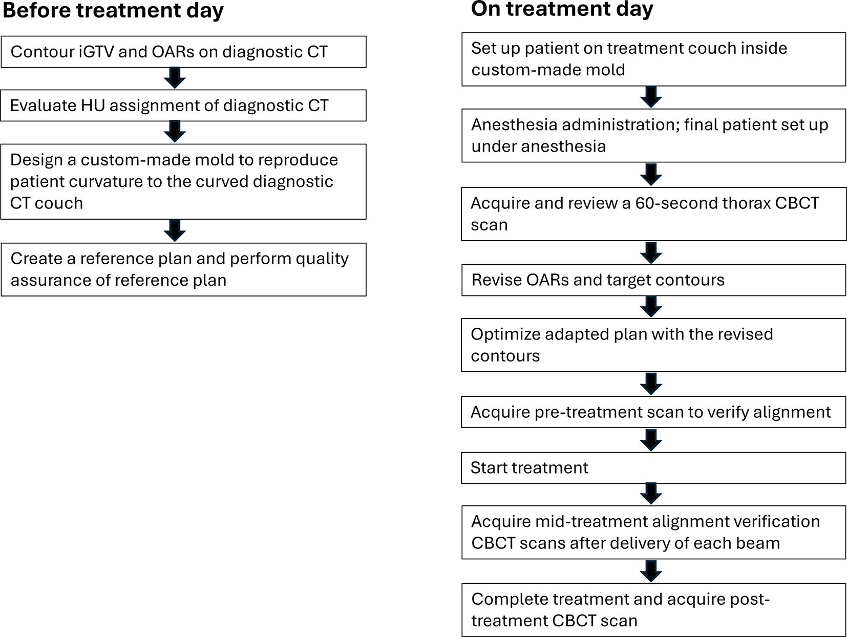
In the CyberKnife M6 radiosurgery system arranged in our hospital, there are two dose calculation algorithms, RayTracing algorithm (TPS-RT) and MC algorithm (TPS-MC). The flowchart of the experiment is shown in Fig. 1, the procedure can be divided into four steps. First, 10 head cases, 10 chest cases, and 10 abdominal cases were collected. Second, the plan was optimized by TPS-RT algorithm with the prescription dose and dose limits, because the TPS-RT algorithm can be completed with less time. Third, the dose re-calculations were implemented on patient CT images by TPS-RT, TPS-MC and ArcherQA-CK to get three different dose distributions (DoseTPS−RT, DoseTPS−MC, DoseArcherQA−CK), where the uncertainty of MC dose calculation was set to 0.5% and the dose calculation resolution was about 1 mm ×1 mm ×1 mm. In this study, the DoseTPS−RT and DoseTPS−MC were calculated on the Precision TPS, DoseArcherQA−CK was obtained with ArcherQA-CK according to the beam information stored in the RT plan files. Finally, the three algorithms were evaluated with the measurements on SRS phantom. In addition, the differences of three dose distributions were compared with each other on 30 cases. In addition, the computational time of two MC algorithms (TPS-MC and ArcherQA-CK) was recorded for comparing the efficiency of different MC algorithms.

Flowchart of the experiment. 10 head cases, 10 chest cases, and 10 abdominal cases were collected firstly. Then, the plan was generated according to the prescription dose and other dose limits, optimized by RT algorithm in TPS. Furthermore, the dose recalculations were implemented by TPS-RT, TPS-MC and ArcherQA-CK algorithms to get three dose distributions. Finally, the differences of three dose distributions were compared

The global 3D gamma analysis (using an absolute dose comparison and 10% low-dose threshold) was completed with PTW Verisoft software, version 5.1 (PTW, Frieburg, Germany), using the following criteria: 2%/1 mm, 3%/1 mm, 2%/2 mm, and 2%/3 mm. In addition, the voxel-wise dose difference within the body was evaluated according to the formula, ΔD = Dg – Dc, where Dg means the dose values of one dose distribution and Dc means dose values of another dose distribution.

In order to further reflect the impact of different dose distributions on the structures, the dosimetric parameters of target area and organs at risk were statistically evaluated and analyzed, including Dmean, D2 and D95 of PTV (here Di means the dose received by i% of PTV volume), as well as Dmean of organs at risk. Paired sample T tests were used to evaluate the statistical significance of all the dose-volume parameters.