Contrast agents (CAs) are commonly used to improve the visibility of anatomical and pathological features in magnetic resonance (MR) scans, thus increasing their diagnostic value. Recommended CA doses have been determined on the basis of efficacy and safety considerations (eg, for gadolinium-based contrast agents [GBCAs], the current standard-of-care suggests a dose of 0.1 mmol Gd/kg). However, several studies indicate that higher doses of CA may be beneficial for detection and evaluation of smaller lesions, or in cases of low CA uptake. Examples include leptomeningeal disease,1,2 metastatic cancer,3–8 multiple sclerosis,9–11 inflammatory demyelinating polyneuropathy,12 and pituitary adenomas.13 Moreover, higher CA dose may facilitate diagnosis in specific cases of meningioma or schwannoma.14

Administration of larger doses of CA involves substantial deviation from standard-of-care procedures and may have safety implications, particularly in the light of recent findings on gadolinium retention and deposition.15,16 Although substantial effort has been devoted to the development of more sensitive MR acquisition schemes17,18 and CAs with higher relaxivity,19,20 a promising avenue to boost image contrast in CA-enhanced MR scans relies on processing of standard images. To this end, it has been suggested that artificial intelligence (AI) approaches, using deep learning (DL) techniques such as convolutional neural network (CNN) or generative adversarial network (GAN) models, could be used on MR images to recover the contrast of a standard dose of GBCA from a lower administered dose,21–27 or to generate an amplified “virtual” contrast, corresponding to higher doses than those normally used, from standard contrast images.28

A neural network for this purpose is typically build by an encoder-decoder architecture reading as input precontrast and postcontrast acquired images and generating as output an image with higher contrast enhancement. The training procedure involves feeding standard contrast images to the network and comparing the output with ground-truth high-contrast images, while adjusting network parameters to minimize a loss function, composed by 2 pixel wise components (mean absolute error in image and Fourier transform domain) and a VGG-19–based perceptual component.

The performance of DL is strongly dependent on the size and quality of the training data set used to model the data distribution. Training data sets should be large enough and sufficiently diverse to avoid bias and enable generalization. They should also include data acquired under a variety of different experimental conditions, sometimes outside standard protocols and typical patient populations. Alas, this kind of data sets is not always available or easily attainable. By way of example, training and validating an AI tool for the prediction of stronger image contrast would require a large set of images acquired at CA doses outside the range of recommended ones in patients with lesions of very different type and conspicuity.

Synthetic data are being increasingly used to implement AI applications in the clinical arena29,30 with the aim of overcoming the scarcity of real-world training data. Synthetic data can be generated from perturbation of real data, or by using physical or AI-driven generative models. Synthetic data can be used to enrich and extend existing data sets, thus improving generalizability and reproducibility of AI approaches, or even to replace real-world data when these are not available.31,32

Here, we describe a DL approach based on synthetic training data to boost image contrast in CA-enhanced MR images. Specifically, we leverage a physical model to simulate different levels of MR image contrast from a GBCA, and we apply the resulting data sets to train a CNN (as originally proposed by Lee et al33) to predict contrast at GBCA doses several times larger than those used in the clinical practice. Unlike previous work on virtual amplification of image contrast,28 our method does not require acquisition of data outside the standard of care and dedicated prospective clinical studies, but can leverage standard data sets. This facilitates enormously the development and extension of AI-based contrast-boosting methods to a variety of applications.

We developed and assessed our AI tool within a translational approach in 2 steps. First, in order to test and refine the simulation strategy, we performed a preclinical study in a rat model of glioma in which we collected a full data set comprising both standard (0.1 mmol Gd/kg) and double-dose images. The virtual double-contrast images generated by a neural network trained with synthetic data were quantitatively and qualitatively evaluated against real double-dose images to assess fidelity and to fine-tune model parameters. Moreover, the validity of the approach was assessed against ex vivo histological data.

In a second step, our AI tool was implemented in a retrospective clinical study, where 1990 examinations from patients with a variety of brain diseases were leveraged to generate synthetic images to train the deep network. Quantitative and qualitative analyses of the AI-enhanced images were presented and discussed in terms of potential benefits for detection and evaluation of small lesions in brain conditions such as metastatic cancer and multiple sclerosis.

MATERIALS AND METHODS Study Design

The purpose of the present study was to train a CNN to virtually double the effects of the CA. To this end, we started from a data set comprising images acquired before CA administration (hereafter named as “pre-CA”) and after 0.1 mmol Gd/kg of GBCA (hereafter named “standard”), and applied the well-established theory of MR signal to compute half-dose images. Pre-CA and half-dose images were then used as input to a DL network (see below), whereas standard-dose images were used as ground-truth to train the network to amplify image contrast. See Figure 1 for a scheme of the proposed strategy.

FIGURE 1:

Scheme of simulation, training, and inference strategy. The simulation process is based on a physical model to generate half-dose images from precontrast and standard-dose images through analytical computation. The training strategy involves the use of precontrast and synthetic half dose images as input for a CNN, whereas standard-dose images are used as output. The network is trained to predict the contrast for a double dose of CA, relative to the CA used to create input images. Finally, the inference strategy uses the trained model to generate a virtual double-dose image from precontrast and standard-dose images. To illustrate this process, a clinical case is presented in the row of images at the bottom.

We entertain the hypothesis that, when applied to standard-dose images, the trained network reliably predicts the contrast that would be generated by a double-dose of CA. This hypothesis was tested experimentally in a preclinical study in laboratory animals, where doses above standard-of-care can be administered to generate ground-truth high-contrast images. Experimental high-dose images in the preclinical model were also leveraged for tuning of hyperparameters. Notably, for the generation of a training data set, our approach requires only pre-CA and standard-dose images, thus making the model applicable in the clinical arena, where data obtained at CA doses above standard-of-care are scarce.

Physical Model

Magnetic resonance image signal in a contrast-enhanced imaging study can be described using a mathematical expression that depends on the following: MR sequence protocol (gradient echo, spin echo, magnetization prepared gradient echo, etc); imaging parameters (echo time [TE], repetition time [TR], and flip angle [α]); tissue parameters (proton density, diamagnetic longitudinal time [T10], transverse relaxation time [T20]); and finally, the local CA's concentration (c), its longitudinal (r1), and transverse (r2) relaxivity.

Focusing on spin echo as a representative example, the MR signal equation can be written as:

S=S01−e−TR1T10+r1ce−TE1T20+r2c

This expression can be linearized with respect to the local concentration c to its first-order approximation. Then, under the assumption of Tofts model34–37 that pharmacokinetic processes are linear in this range of doses (between half and full dose) and that local concentration scales linearly with the dose (ie, the local concentration at half dose is one half the concentration at standard dose), the MR signal of half dose images can be calculated as follows:

Shalf dose≅Spre+fS0TETRT10T20r1r2chalf dose=Spre+Sstandard dose−Sprechigh dosechalf dose=Spre+Sstandard dose−Spre2

where S is the MR signal precontrast, at half dose or standard dose as indicated in the subscripts, and c is the local concentration of CA at half dose or standard dose as indicated in the subscripts.

Data Sets Preclinical Study

Procedures were conducted according to the national and international laws on experimental animal research (L.D. 26/2014; Directive 2010/63/EU) and under a specific Italian Ministerial Authorization (project research number 384/2021-PR).

Forty-eight male Wistar rats (Charles River Laboratories, Calco, Italy), aged 7–8 weeks (250–300 g body weight), underwent a surgical procedure to induce a glioma by orthotopic injection of C6 rat glioma cells.38,39 Rat glioma cells were supplied by Sigma Aldrich (ECACC) and cultured in DMEM F-12 medium supplemented with 10% fetal bovine serum, 2 mM glutamine, 100 IU/mL penicillin, and 100 μg/mL streptomycin. For tumor induction, cells were collected, washed 2 times with PBS, and finally a total number of 106 cells were resuspended in 10 μL of DMEM F-12.

Rats were subcutaneously injected with carprofen (5 mg/kg) 1 hour before the surgery. Anesthesia was induced with sevoflurane gas and then maintained systemically with Rompun (5 mg/kg) and Zoletil (20 mg/kg). Each rat was then mounted on the stereotaxic apparatus to identify the injection site (0.8 mm anterior, 3.2 mm lateral to bregma and 6 mm ventral to bone). The injection was carried out by using a Hamilton syringe with needle's tip (25 gauge) cut in order to yield more accurate cells release, at a rate of 1 μL/min. The volume was released manually via repeated administrations of 1 μL each 60 seconds. The needle was carefully and slowly removed 15 minutes after the end of the injection to avoid cell dispersion.

In a time window ranging between 7 and 16 days after tumor induction, 44 animals that survived tumor induction procedure and did not show severe clinical signs40 underwent contrast-enhanced MR imaging for a total of 2/3 sessions. Each examination was recorded 24–48 hours apart.

A total of 121 examinations (acquired at 3 T or 7 T and pooled together) were collected from the 44 animals, each composed of a pre-CA, a standard-dose image, and a double-dose image. For each examination, an additional image corresponding to the administration of half the standard dose (“half dose”) was generated applying the simulation strategy described previously.

Magnetic resonance imaging was performed on 2 different preclinical scanners (Bruker Biospin, Ettlingen, Germany): Biospec 47/30 operating at 3 T equipped with a 4-channel rat head surface coil and Pharmascan 70/10 operating at 7 T equipped with a quadrature volume rat head coil. Two different scanners were used to test the effects of field strength on the performance of our AI approach. Each animal underwent 1 or 2 sessions for each scanner for a total of 3 sessions at most.

The contrast-enhanced MR protocol consisted of the acquisition of spin echo T1-weighted images before CA administration, after the first intravenous administration through the caudal vein of ProHance (Bracco Imaging, Milan, Italy) at “standard dose” 0.1 mmol Gd/kg and after a second administration of 0.1 mmol Gd/kg. The CA was administered after dilution in saline to a concentration of 100 mM at an injection rate of approximately 1 mL/min. The first postcontrast acquisition started with the first injection of CA. The second postcontrast acquisition started immediately after the end of the first scan, at the time of the second injection. On first approximation, pharmacokinetic effects that may occur in the time window between the administration of the 2 doses were not taken into account, and the second postcontrast acquisition was assumed to correspond cumulatively to a “double-dose” acquisition. This scheme increases statistical power, making it possible a within-subject analysis, thus reducing the number of subjects, according to the principles of 3R.

T1-weighted images were acquired with the parameters reported in Table 1.

TABLE 1 - MRI Acquisition Parameters Used in the Preclinical and Clinical Protocols Protocol Preclinical Clinical Machine and B0 Bruker Pharmascan 70/10 Scanner 7 T Bruker Biospec 47/30 Scanner 3 T MRI Philips Panorama 1 T, MRI Philips Prodiva CX 1.5 T, MRI GE Signa Twin 1.5 T, MRI Philips Achieva XR 3 T Modality T1-weighted T1-weighted T1-weighted Sequence 2D spin echo 2D spin echo Mainly 2D spin echo TR 360 ms 400 ms 476 ms (±100 ms) TE 5.51 ms 14.3 ms 11.9 ms (±3.6 ms) FOV 32 × 32 mm 32 × 32 mm — Matrix size 256 × 256 256 × 256 — Planar resolution 125 × 125 μm 125 × 125 μm 478 × 478 μm (±143 × 143 μm) Slice thickness 0.75 mm 1.2 mm 4 mm (±1 mm)

B0, the static magnetic field; TR, repetition time; TE, echo time; FOV, field of view.

Clinical Study

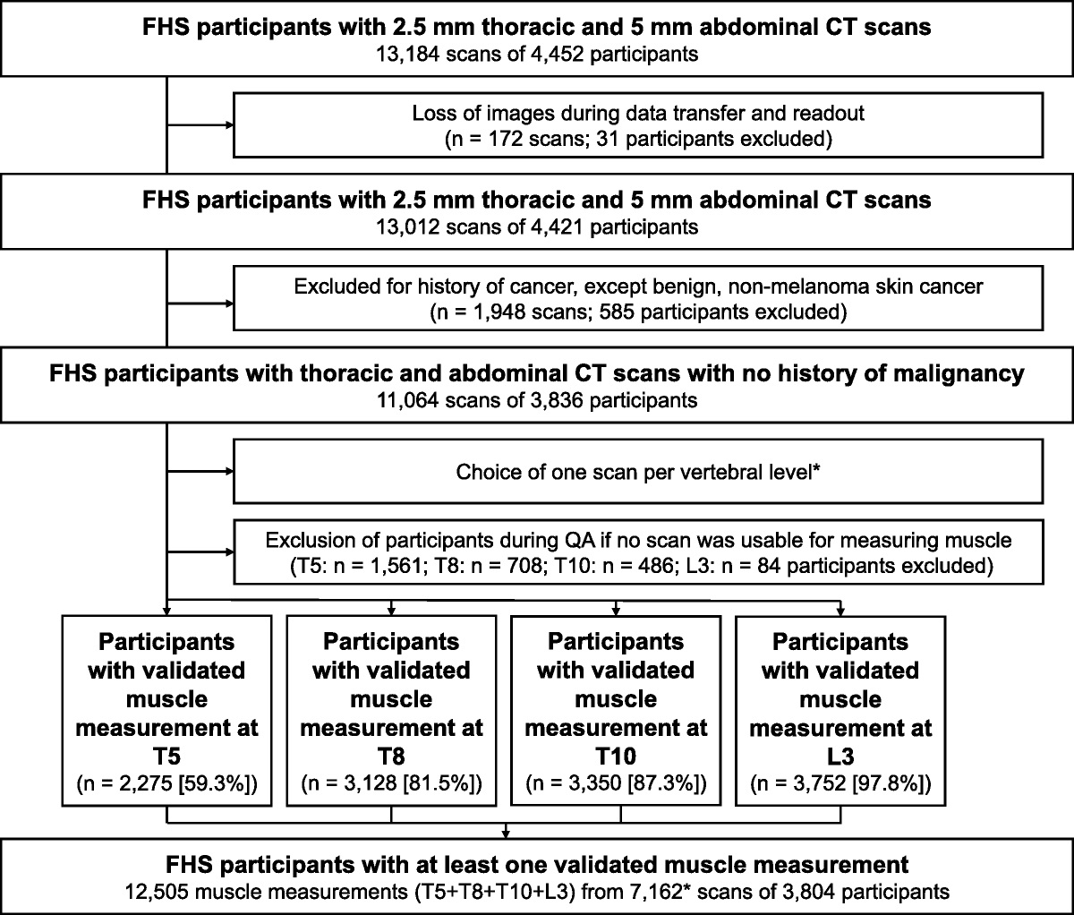
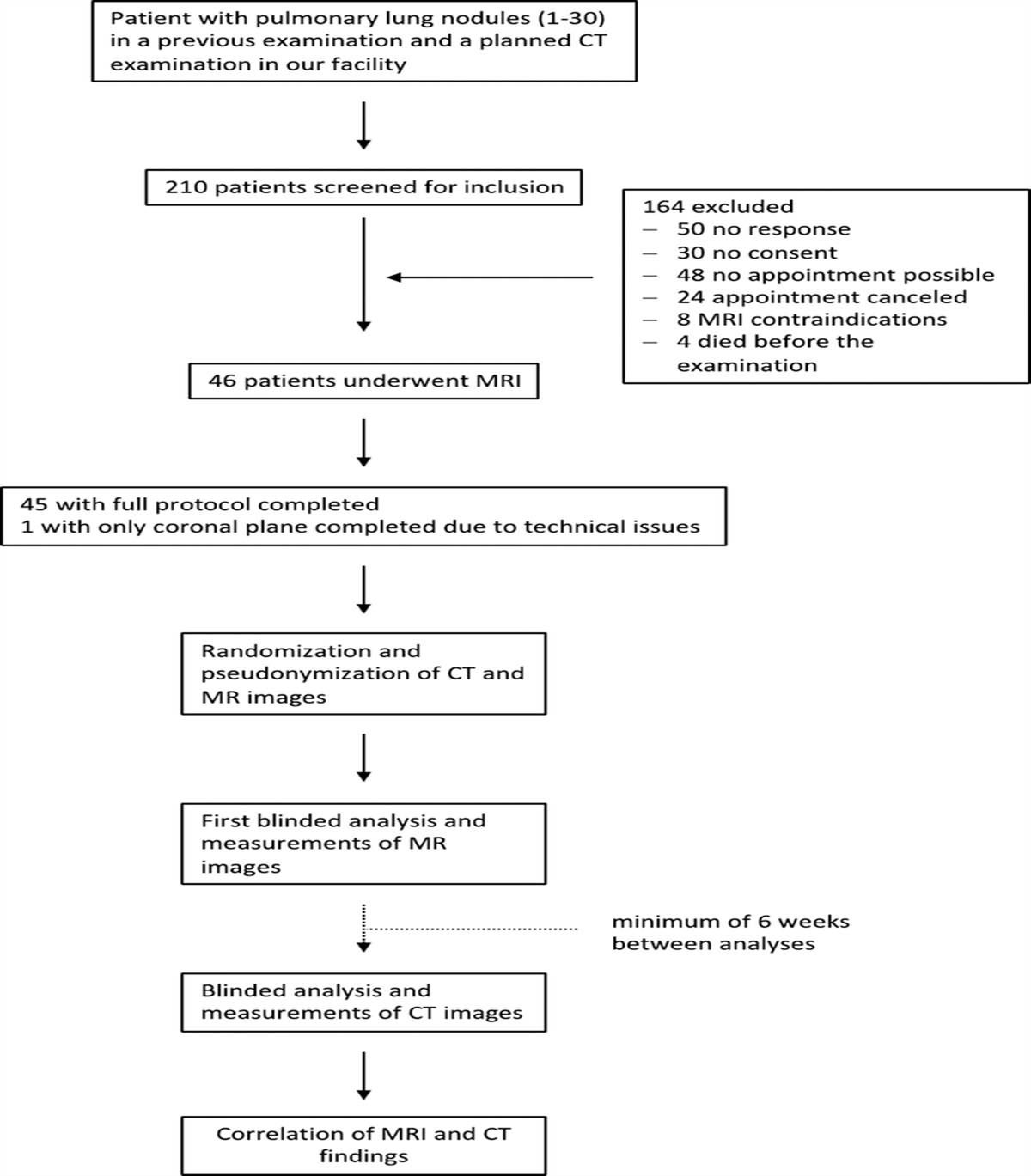
A total of 4711 central nervous system MR imaging examinations, acquired between January 2012 and March 2020 at Centro Diagnostico Italiano (CDI, Milan, Italy; Bracco Group), were considered for inclusion in this retrospective monocentric study approved by the institutional review board (registration number 181/2020). Patients older than 18 years who underwent MR contrast-enhanced brain scans, including a pre-CA and postcontrast image with the same repetition time, axial orientation, and acquisition matrix, were considered for inclusion. The flow diagram (Fig. 2) details the exclusion mechanisms. One thousand nine hundred ninety (of the 4711 collected examinations) with a variety of brain pathologies (eg, meningioma, multiple sclerosis, neurinoma, etc) were included in the study.

FIGURE 2:

Exclusion flowchart for clinical data set.

The acquisitions were performed using either General Electric or Philips scanners operating at different magnetic field strengths ranging between 1 T and 3 T (MRI Philips Panorama 1 T, MRI Philips Prodiva CX 1.5 T, MRI GE Signa Twin 1.5 T, and MRI Philips Achieva XR 3 T). Most of collected T1-weighted images were 2D spin echo sequences acquired with the parameters reported in Table 1.

Image Preprocessing

Contrast-enhanced images and the corresponding pre-CA acquisitions were geometrically aligned using the SimpleElastix41 software package with a nonrigid registration procedure. A visual quality check was finally performed through a graphical user interface (GUI) internally developed with PAGE (an open-source program) to exclude the presence of artifacts in the generated images (eg, related to the failure of the coregistration procedure).

Magnetic resonance imaging signal was normalized to have the pre- and half-dose images mapped onto the [0, 1] range, by dividing each image by the maximum value of the synthetic half dose image. Hence, signal in the standard- and double-dose image can exceed the value of 1.

Deep Network Structure Description of Network

We implemented a U-net like encoder-decoder convolutional neural network as originally described by Lee et al,33 and as represented in Figure 3. The proposed network consists of an encoder and a decoder. The encoder is a series of 3 convolutional and pooling layers that down-sample the input image while extracting features from it. The decoder is a series of 3 up-sampling and convolutional layers that reconstruct the original image size. Each level of the encoder and decoder path consists of a residual block with 2 sequential 3 × 3 convolution layer with batch normalization and rectified linear unit (ReLU) activation and a “shortcut” connection consisting of a 1 × 1 convolution with ReLU and batch normalization. The output of the 3 × 3 convolution layers is added to the output of the 1 × 1 convolution creating the residual connection. In the encoder, each stage is followed by a 2 × 2 max pooling layer, while 2 × 2 up-sampling layers are used in the decoder to increase the spatial resolution. Similarly to the original U-net architecture, skip connections are added to connect corresponding levels of the encoder and decoder paths. The number of channels used in each convolution layer is shown in Figure 3. The resolution of the input layer is 256 × 256. The cost function (described below) compared the prediction and the reference ground-truth full-dose image, which enabled the optimization of the network parameters.

FIGURE 3:

Deep learning network architecture used in this work. This model is an encoder-decoder convolutional neural network consisting of a series of 3 encoder steps and a series of 3 decoder steps.

Network Training

Using pairs of pre-CA and simulated half-dose images as input and standard-dose images as ground-truth, the network was trained to predict standard-dose images.

The data set was split in training set (70%), validation set (20%), and test set (10%) to train and validate the DL model. Data augmentation, consisting of rotations, flips, was applied to images of the training set to avoid overfitting and ensure the robustness of the model. A key step in the data augmentation is the adjustment of noise levels to be added to half-dose images to match realistic signal-to-noise and contrast-to-noise levels. To this end, we added normally distributed noise with zero mean and tunable standard deviation (SD) to the simulated images. Normally distributed noise was added, rather than Rician noise, since Rice distribution approaches a Gaussian one at sufficiently high signal-to-noise ratio (SNR) (>2).42 Since the level of added noise affected the performance of the network, this parameter was treated as hyperparameter.

Stochastic gradient descent and back-propagation were used to optimize the network weights and bias. A 3-component composite loss was used as cost function: mean absolute error (MAE), MAE in the Fourier transform space, and the perceptual loss43 based on the VGG-1944 network pretrained on the ImageNet data set and cut at the fourth pooling layer. To match the size of our input with that of VGG-19 network (ie, 3 channels input layer, being trained on RGB images) for each image a 3 channels tensor is created by repeating the grayscale image 3 times. The 3 components of the loss were normalized to balance their weight during training. The normalization procedure consisted of training a network with only one loss component and measuring its mean value. This mean value was then used to normalize each loss component so that the mean value was set to one. Then, 3 weights were included in the loss function (“a,” “b,” “c”) to modify the relative contribution of each component and to study their effect on the final image quality (IQ). Specifically, the following hyperparameters were subjected to the tuning process: weight of MAE as pixelwise loss component (“a” = 0.5, 1 or 2) and weight of perceptual loss component (“c” = 1, 2, or 5). Similarly, different values of noise SD (ie, 0.0075, 0.01, 0.015, 0.03) were investigated. For each hyperparameter setting (weight of loss components and SD of noise), 5 repetitions of training and testing were carried out after shuffling training, validation, and test data sets. Training was performed with 250 epochs of stochastic gradient descent using ADAM as optimizer with learning rate 0.01 and decay 0.001.

Each trained network was then applied to predict virtual double-dose images using pre- and standard-dose images as input.

Preclinical Evaluation

Similarity of virtual double-dose and standard-dose images against real double-dose images was assessed using peak SNR (PSNR) and structural similarity index (SSIM),45,46 respectively, a measure of voxel-wise differences (errors) and nonlocal structural similarity. The metrics were computed for both standard-dose images and the virtual double-dose images against the ground-truth, that is, the experimental double-dose image, to study the similarity improvement obtained by the CNN. Data are shown as average values ± standard error. The significance of statistical difference was assessed by a Student t test.

Clinical Evaluation

As detailed in Table 2, 2 evaluation studies were performed: the first one aimed at quantitatively assessing the increment of contrast-to-noise ratio (CNR) and lesion-to-brain ratio (LBR), and the second one aimed at qualitatively scoring the visibility of small lesions.

TABLE 2 - Description of the Clinical Evaluation Studies Aspect Study 1 Study 2 Rationale To quantitatively assess the increment of CNR and LBR and to qualitatively score DC, CE, AS, and IQ on a 5-point Likert scale To qualitatively score, the visibility of small lesions on a 5-point Likert scale Image data set presented to radiologist A total of 60 patients (for a total of 120 cases/images: 60 true standard dose and 60 virtual double dose) were randomly selected and then included in the present study A total of 30 patients (for a total of 60 cases/images: 30 true standard dose and 30 virtual double dose) were randomly selected and then included in the present study Pathologies included • Meningioma (n = 10)
• Multiple sclerosis (n = 10)
• Glioblastoma (n = 10)
• Astrocytoma (n = 10)
• Metastases (n = 10)
• Angioma (n = 10) • Metastases (n = 15)
• Active multiple sclerosis (n = 15) Readers numbers 2 board-certified neuroradiologists (I.L.T. and M.P. with 19 and 1.5 years of experience, respectively) not blinded to image source dose (ie, standard dose or virtual double dose) 3 board-certified neuroradiologists (N.C., C.D.G., and G.S. with 40, 44, and 47 years of experience), respectively, blinded to the image source dose (ie, standard dose or virtual double dose). Question asked to radiologists • During the quantitative evaluation: to place on each case a first ROI in the largest homogenous enhancing area of the lesion and a second ROI in the contralateral cerebral parenchyma (avoiding large blood vessels)
• During the qualitative evaluation: to grade for each case DC, CE, AS, and IQ on a 5-point Likert scale To qualitatively grade for each case visibility, degree of delineation and brightness of small enhancing structures on a 5-point Likert scale
Study 1

For the quantitative and qualitative evaluation of model performance, a subset of 60 patient scans were randomly selected and included in the test set: 22 males and 38 females; mean age, 56 ± 15 years (min = 27, max = 81 years); scanners: MRI Philips Panorama 1 T (n = 11), MRI Philips Prodiva CX 1.5 T (n = 27), MRI GE Signa Twin 1.5 T (n = 19), and MRI Philips Achieva XR 3 T (n = 3); even distribution of pathologies (meningioma [n = 10], multiple sclerosis [n = 10], glioblastoma [n = 10], astrocytoma [n = 10], metastases [n = 10], angioma [n = 10]). A total of 120 (60 true standard dose and 60 virtual double dose) cases were presented to 2 board-certified neuroradiologists (I.L.T. and M.P. with 19 and 1.5years of experience respectively). During the quantitative evaluation, the readers independently placed the first region of interest (ROI) in the largest homogenous enhancing area of the lesion and a second ROI in the contralateral cerebral parenchyma (avoiding large blood vessels). The percentage variation of CNR and LBR of virtual double dose with respect to standard dose was computed for each case with at least 1 enhancing lesion, according to the formulae:

CNR=SIlesion−SIbrainSDbrain

LBR=SIlesionSIbrain

where SIROI and SDROI, respectively, denote the average signal intensity (SI) and its SD in a given ROI (where ROI = lesion, brain). Data are presented as average values ± standard error. During the qualitative evaluation, the readers independently graded diagnostic confidence (DC), clarity of the enhancement (CE), artifact suppression (AS), and IQ on a 5-point Likert scale. Average scores and related 95% confidence intervals were both calculated across readers and type of the image.

Study 2

In a second run of clinical evaluation, the original standard-dose images and the virtual double-dose images were qualitatively evaluated by neuroradiologists N.C., C.D.G., and G.S. with 40, 44, and 47 years of experience, respectively, blinded to the image source. The readers independently graded visibility, degree of delineation, and brightness of small enhancing structures (larger diameter on average 3.54 ± 1.05 mm; min = 1.04 mm and max = 5.47 mm) on a 5-point Likert scale on 15 cases of metastases (larger diameter on average 3.70 ± 1.26 mm; min = 1.04 mm and max = 5.47 mm) and 15 cases of active multiple sclerosis (larger diameter on average 3.37 ± 0.81 mm; min = 2.33 mm and max = 5.12 mm). Average score across readers and type of the image was computed using 2-tailed t test, with a 5% level used for confidence intervals and statistical significance.

RESULTS Preclinical Results

Figure 4 shows representative examples of experimental pre-CA, standard-dose, and double-dose images compared with AI-generated virtual double-dose images for 2 subjects at 2 different magnetic field strengths (7 T, top row, and 3 T, bottom row). At both fields, virtual double-dose image contrast is substantially enhanced compared with that of standard-dose images, with good delineation of lesion boundaries and tumor heterogeneity in qualitative agreement with the experimental double-dose images. The enhancement of the virtual double-dose image contrast is also apparent in the lateral ventricles and in cortical blood vessels.

FIGURE 4:

Representative example of pre-CA (A), standard-dose image (B), real double-dose image (C), and virtual double-dose image (D), and difference image between real double-dose and virtual double-dose (E) from an examination acquired at 7 T (top row) and 3 T (bottom row).

The lesions displayed in Figure 4 are characterized by well-defined hyperintense rims. In contrast, Figure 5 presents MR images of a tumor infiltrating subcortical areas, where lower CA uptake makes it difficult to identify tumor boundaries in the standard-dose image (Fig. 5B). Visual inspection of real and virtual double-dose contrast (panel “c” and “d,” respectively) shows substantial enhancement of CNR in brain regions away from the point of implantation. Importantly, histological examination of postmortem tissue demonstrates correspondence of virtual contrast with neoplastic tissue in the infiltrated regions. Additional illustrative comparisons of real and virtual double-dose contrast images with histological slices are reported in the Supplementary Material section, https://links.lww.com/RLI/A839.

FIGURE 5:

Representative example of pre-CA (A), standard-dose image (B), real double-dose image (C), virtual double-dose (D), and histology (E).

Focusing on CNN optimization, as described in the Methods section, a small albeit appreciable influence of the weights “a,” “b,” and “c” was observed (up to 1 dB and 0.5 percentage points for PSNR and SSIM, respectively). Parameters were tuned to increase metrics values of double virtual dose against acquired virtual dose as much as possible. The best result was obtained setting “a” = 0.5 and “c” = 1. The second best results were obtained with “a” = 2 and “c” = 5.

The effect of the noise level is shown in Figure 6, where representative images at increasing noise are reported, as well as a quantitative evaluation based on SSIM. The SSIM was chosen as a metric because it is known to better represent changes in structural information compared with pixel-wise metrics based on absolute errors (such as MSE or PSNR). According to SSIM, the higher the noise, the higher the similarity between acquired and virtual double dose. Visually, at low noise level, the image shows a texture that differs from ground-truth, showing artificial fluctuations of gray levels in the healthy brain parenchyma. At increasing noise fluctuations, results smoothed up to a slightly over blurring for the highest values. The best compromise appears to be the intermediate levels of noise equal to 0.015 for both magnetic field strengths, for which the SSIM values are higher than those obtained with standard dose, and at the same time the blurring is moderate.

FIGURE 6:

Representative example of double-dose image (A), virtual double-dose with noise 0.0075 (B), 0.01 (C), 0.015 (D), and 0.03 (E). SSIM at 7 T (F) and SSIM at 3 T (G). *P < 0.05. **P < 0.01. ***P < 0.

After model optimization, quantitative comparison of the experimental and virtual double-dose images was performed on a test data set comprising 13 randomly selected subjects. We used 2 different metrics, PSNR and SSIM, and results were averaged over 5 repetitions of training, shuffling training, validation, and test sets. Figure 7 shows the summary statistics across all subjects included in the test sets for both indices at 3 T and 7 T. It should be noted that the metrics were conservatively computed over the entire image, without prior segmentation of the tumor lesion. Virtual double-dose images show high degrees of similarity to real double-dose images for both PSNR and SSIM (29.49 dB and 0.914 at 7 T, respectively, and 31.32 dB and 0.942 at 3 T) and highly significant improvement over standard-dose images at both field strengths (light gray bars).

FIGURE 7:

Evaluations using quantitative nonsubjective similarity metrics (PSNR [dB] panel A and SSIM panel B) of acquired standard-dose and virtual double-dose compared against acquired double-dose ground-truth on testing data sets. *P < 0.05. **P < 0.01. ***P < 0.

Clinical Results

The network architecture and training procedures that were optimized and validated on the preclinical data set were subsequently applied to a large set of clinical data comprising a variety of brain conditions. Examples of representative cases are reported in Figure 8, where experimental pre-CA and standard-dose images are compared with virtual double-dose ones. Consistent with the preclinical findings, virtual double-dose contrast improves delineation of lesion boundaries and enhances tumor texture compared with standard-dose images, while leaving bright the pre-CA T1 perilesional hyperintense signal. Strong contrast enhancement is also observed in blood vessels, which appear as prominent features in the virtual double-dose contrast images.

FIGURE 8:

Representative clinical cases of astrocytoma, metastases, multiple sclerosis, and glioblastoma, respectively, from top to bottom. A and D, Pre-CA. B and E, Standard dose postcontrast image. C and F, Virtual double-dose image. The red square indicates the zoomed area showed in panels D, C, and F.

The virtual double-dose images were quantitatively and qualitatively evaluated in 2 reading studies, against the original standard-dose acquisition.

The quantitative assessment of the degree of the amplification of virtual double-dose contrast images was evaluated for a subset of 60 patients with various brain pathologies. Results are summarized in Figure 9. The percentage gain in CNR (virtual double dose contrast vs standard dose) and LBR are shown in Figure 9A and Figure 9B, respectively, for the ROIs selected by 2 independent expert readers. Contrast-to-noise ratio and LBR are consistently increased by an average 155% and 34%, respectively, with no significant differences for the 2 readers. The qualitative scores assigned by the 2 neuroradiologists indicated that the CE is maintained acceptable to good for both standard dose and virtual double dose according to reader 1 and increased by 0.5 points in virtual double dose with respect to standard dose according to reader 2 (see Table 3). Both the 2 readers perceived also DC, IQ, and AS not compromised in the virtual double-dose image with respect to that of the standard-dose image. The average qualitative score and the related confidence of interval exhibit a perception acceptable to good for the virtual double-dose contrast as well as for standard-dose image (see Table 3).

FIGURE 9:

Contrast evaluations using quantitative nonsubjective metrics (%CNR and %LBR) of virtual double-dose images compared against standard-dose acquisitions on testing data sets.

TABLE 3 - Average Scores of CE, DC, AS, and IQ for the Selected Test Sample (n = 60 Standard Dose and n = 60 Virtual Double Dose) Reader ID CE DC AS IQ Standard Dose Virtual Double Dose Standard Dose Virtual Double Dose Standard Dose Virtual Double Dose Standard Dose Virtual Double Dose Reader 1 3.92 (3.8, 4.1) 3.85 (3.7, 4.0) 3.92 (3.7, 4.1) 3.33 (3.1, 3.6) 3.30 (3.1, 3.5) 2.45 (2.2, 2.7) 3.95 (3.8, 4.1) 3.15 (2.9, 3.4) Reader 2 3.50 (3.2, 3.8) 4.02 (3.8, 4.3) 3.62 (3.4, 3.9) 3.40 (3.2, 3.6) 3.58 (3.3, 3.8) 3.17 (2.9, 3.4) 3.83 (3.6, 4.1) 3.45 (3.2, 3.7)

Grades are expressed on a 5-point Likert scale ranging from 1 (poor) to 5 (excellent). Mean values are reported, with the corresponding standard deviations between parentheses.

The qualitative assessment in terms of visibility, degree of delineation, and brightness of small low-enhancing lesions was performed in a subset of 30 patients, 15 of whom affected by multiple sclerosis and the remaining by multiple metastases. As detailed in Table 4, the virtual double-dose images were preferred by all 3 readers. On average between readers, standard-dose images were graded 3.51 of 5 (average to good), whereas virtual double-dose images were graded 4.46 of 5 (good to excellent). Two representative examples of small lesion virtually enhanced by our model are shown in Figure 10.

TABLE 4 - Average Scores of Visibility, Delineation, and Brightness of Small Contrast Enhancing Lesion for the 30 Cases of the Selected Test Sample Standard Dose Virtual Double Dose Standard Dose vs Virtual Double Dose Counts Reader average 3.51 (0.62) 4.46 (0.69) P << 0.001* 90 Reader 1 3.67 (0.55) 4.63 (0.56) P << 0.001* 30 Reader 2 3.63 (0.61) 4.63 (0.61) P << 0.001* 30 Reader 3 3.23 (0.63) 4.10 (0.76) P << 0.001* 30 R1 vs R2 P = 0.77 P = 1 NA 30 R1 vs R3 P < 0.05* P < 0.001*