Kidney diseases have emerged as a growing global health concern, with an increasing prevalence and detrimental impact on individuals' quality of life.1 They strongly reduce life expectancy, and it is considered that chronic kidney disease affects as many as 10%–15% of the population worldwide. Among the structures within the kidneys, glomeruli contribute to blood filtration and regulate its composition.2 Consequently, any impairment in their microvascular anatomy can lead to significant disruptions in kidney function. Chronic ailments such as high blood pressure, diabetes mellitus, and autoimmune diseases can adversely affect the glomeruli, resulting in their destruction and subsequent loss of filtration capability.3–5 Progressive sclerosis of glomeruli is also a universal feature of any chronic kidney disease. However, current clinical imaging techniques cannot visualize individual glomeruli.6–9 The significant challenge lies in the diameter of human glomeruli, which is approximately 200 μm10 and falls below the resolution limit of most medical imaging methods. Therefore, the glomerulus function is indirectly studied in the clinic by blood or urine tests that only provide access to the global glomerular filtration rate11–13 or biopsies.14,15

Ultrasound localization microscopy (ULM)16–18 is an acoustic superresolution imaging technique that tracks intravascular ultrasound contrast agents (microbubbles)19,20 to map the organ's microcirculation.21–23 This technique has achieved unprecedented resolution in living animal24–27 and in human organs,28–30 including studies with standard ultrasound scanners.31 Although ULM provides detailed microvascular maps, it still cannot visualize the functional units within organs. This limitation partly arises from the challenge of distinguishing very slow-moving microbubbles within capillary beds.32 To address this, our team developed a novel method called “sensing ULM (sULM),” which uses microbubbles as sensors of their immediate environment. The sULM enhanced accuracy by classifying microbubble motion patterns corresponding to expected microscopic structures. By applying sULM on human kidney allografts, we have successfully observed the kidney's glomeruli.33 Still, the feasibility of visualizing glomeruli in their natural kidney environment has yet to be determined. Native kidneys, when imaged with ultrasound, present greater complexity than allografts. The native position of the organ is more profound and, therefore, more affected by wave attenuation and respiratory movements.34 On the contrary, the fixation of kidney grafts within the retroperitoneal space35 leads to their quasi-immobility, which enables longer and uninterrupted imaging sessions,31,33 an important factor for the proposed sULM technique.36

This study aimed to evaluate the ability of sULM to visualize glomeruli in native human kidneys in vivo. A secondary objective was to compare the sULM parameters (acquisition time, depth, and frame rate) between native kidneys and kidney allografts and their consequence regarding glomeruli detection.

MATERIALS AND METHODS Ethics Approval

This study was approved by the Ethics Committee of the French Society of Radiology (CERF, reference numbers CRM-2304-345 and CRM-2203-240). Patients recruitment occurred in our genitourinary university center.

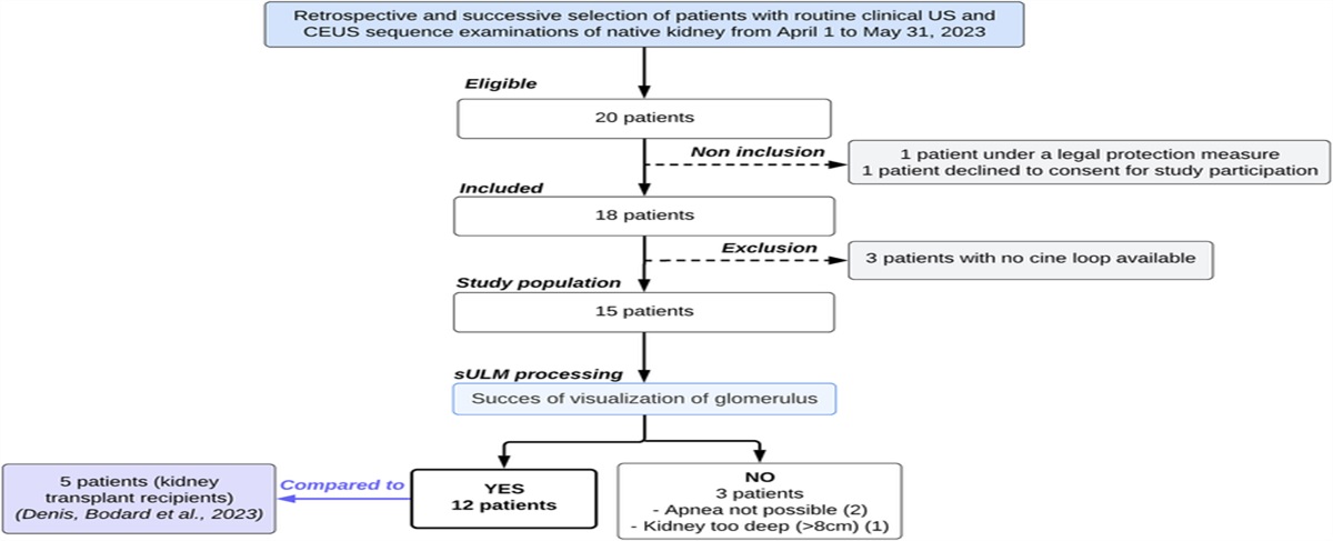
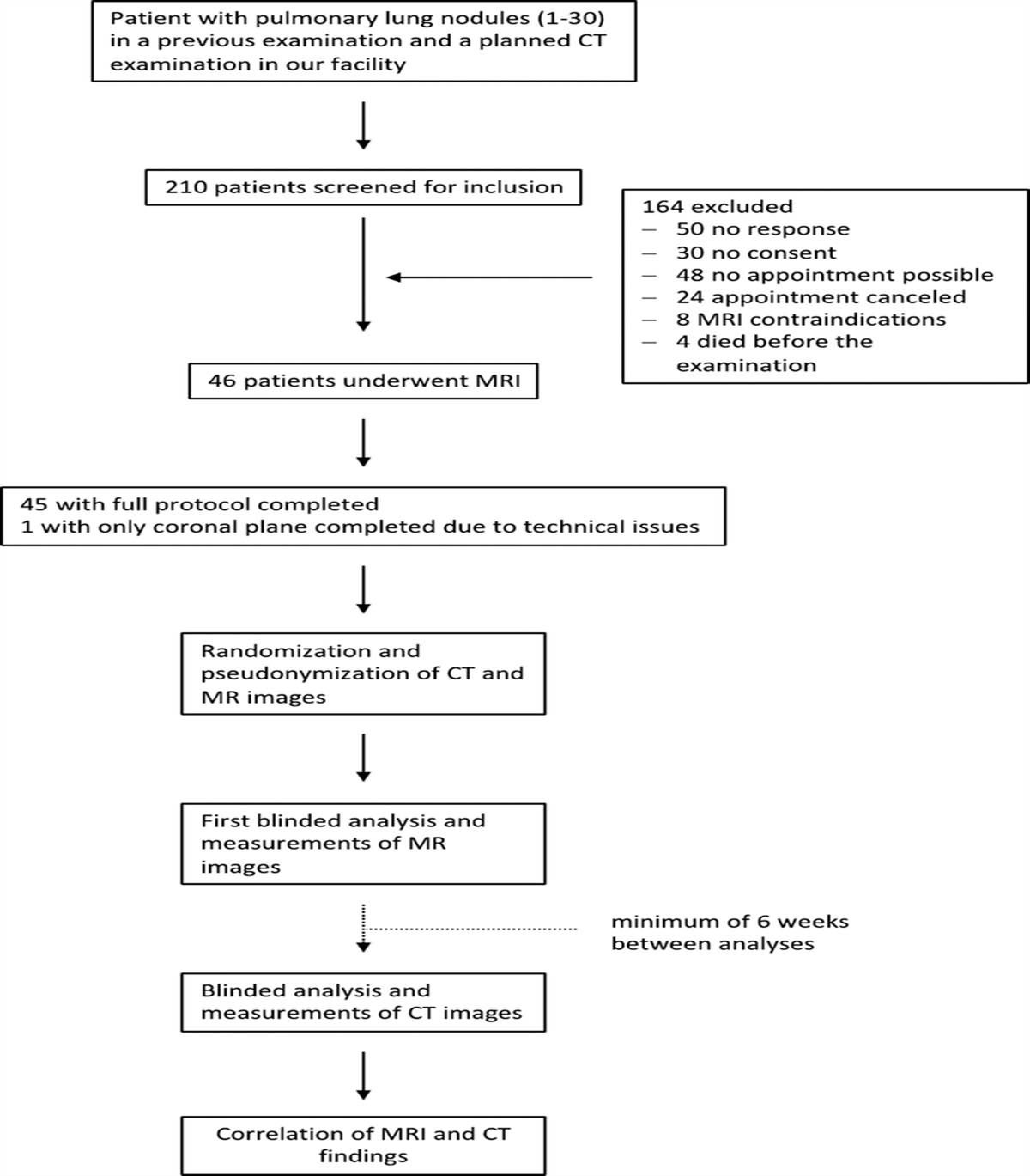
Population Study

From April 1 to May 30, 2023, 18 patients undergoing clinical ultrasound examinations of their native kidneys, including contrast-enhanced ultrasound (CEUS), were retrospectively included. No additional experimental procedures were added. We also included 5 kidney transplant patients from our previous study in which we demonstrated that the sULM was possible to visualize the glomeruli of kidney allografts.33 Both groups were treated with the same postprocessing sULM algorithms detailed below. Figure 1 summarizes the flowchart of the study.

FIGURE 1:

Study flowchart.

CEUS Acquisition

Contrast-enhanced ultrasound was performed using a clinical ultrasound scanner Aplio i800 (Canon MS, Nasu, Japan) in contrast mode with a convex abdominal probe i8cX1 (3 MHz, Canon, bandwidth [1.8–6.2] MHz) as part of routine clinical examinations of patients. No additional examinations have been added. Patients were positioned in the lateral decubitus position and held their breath during the acquisition. A bolus of 1.2 mL of contrast agent (SonoVue; Bracco, Milan, Italy, containing 8 μL of sulfur hexafluoride/mL) was injected intravenously. This dosage is consistent with standard clinical practices but introduces a high concentration of microbubbles into the bloodstream. We mitigated this using data acquired after a sufficient delay (a few minutes, as reported in Table 1). This time delay allowed the microbubble concentration to decrease adequately, thereby achieving the prerequisite of significantly separated microbubbles for effective sULM. The mechanical index was reduced to 0.08 to preserve microbubble integrity during acquisition. The frame rate and the duration depended respectively on the kidney depth and the time of the patient's breath-holding.

TABLE 1 - sULM Measurements and Parameters Patient Number Deep Min* (mm) Deep Max† (mm) Frame Rate (fps) CEUS Loop Duration (s) Time After SonoVue Injection (min:s) Kidney Surface Explored (cm2) No. Microbubbles Localizations/cm2‡ No. Track Detected/cm2‡ No. Glomeruli Detected/cm2‡ Native kidneys 45 [29–87] 98 [29–142] 41 [28–78] 23 [15–36] 4: 55 [2: 23–8: 54] 22 [7–30] 2366 [523–8862] 148 [32–486] 16 [6–31]  1 41 99 49 33 8: 54 21 2359 156 18  2 45 110 32 36 5: 07 24 2670 153 16  3 35 86 39 26 5: 38 19 1396 89 20  4 45 111 43 21 5: 19 29 954 71 11  5 36 85 78 19 3: 26 7 8862 486 31  6 46 73 39 24 6: 02 14 3330 203 31  7 87 (too deep) 142 28 15 X X X X None  8 40 99 39 27 4: 37 28 2799 178 12  9 35 86 35 19 2: 23 18 1044 64 15  10 38 92 49 Impossible apnea X X X X None  11 41 100 39 29 2: 26 24 2826 232 14  12 51 124 32 18 7: 12 29 523 32 7  13 51 123 43 15 3: 29 26 893 43 6  14 46 111 39 25 4: 29 30 743 64 8  15 29 29 38 Impossible apnea X X X X None Kidney allografts 32 [21–52] 87 [58–124] 36 [14–64] 143 [69–183] 5: 82 [5: 13–7: 13] 28 [8–48] 11,971 [3515–18,745] 679 [217–1046] 33 [18–55]  16 24 99 22 177 5: 13 40 18,745 891 27  17 21 58 64 109 5: 33 8 15,411 1046 55  18 28 58 56 179 5: 48 9 15,084 928 47  19 34 97 24 69 5: 43 36 3515 217 21  20 52 124 14 183 7: 13 48 7100 316 18

*Depth (distance probe − renal cortex).

†Depth (distance probe − deepest part of the kidney).

‡Normalized by kidney area (cm2).

sULM, Sensing ultrasound localization microscopy; fps, frames per second; CEUS, contrast-enhanced ultrasound.

Data Collection

Data collection encompassed demographic, clinical, ultrasound, and CEUS parameters. Demographic information, including age, sex, and body mass index, was recorded for each participant. Clinical variables were also included, such as the estimated glomerular filtration rate, the presence of high blood pressure, diabetes mellitus, or underlying kidney diseases. Details of any medications targeting renal function were also documented. Supplementary Table S1 (https://links.lww.com/RLI/A893) summarizes the demographic and clinical characteristics of the study population.

Ultrasound and CEUS data, including renal depth, frame rate, and breath-holding duration, were reported in Table 1. The Supplementary Material (https://links.lww.com/RLI/A894) section provides information on CEUS acquisition.

All data were anonymized and subsequently analyzed with Matlab.

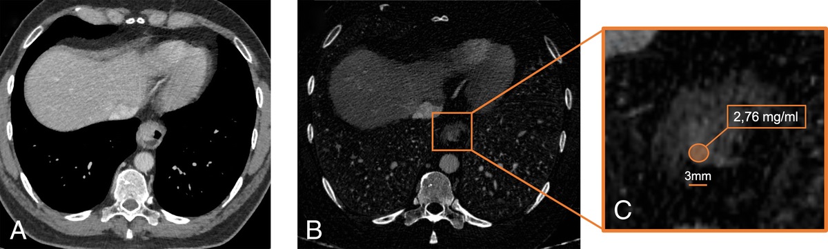
sULM Postprocessing, Glomeruli Detection, Visualization, and Count

Contrast-enhanced ultrasound loops (Fig. 2B) were divided into blocks of 200 frames each. A succession of steps was then applied on each block to generate an ULM density map (number of microbubbles tracked per pixel). The first step involved a bandpass first-order temporal filter, with a frequency ranging from 0.5 to 5.5 Hz that highlights microbubbles with a specific velocity, that is, a temporal oscillation within the pixel. In vessels with fast blood flow, amplitude oscillations will be closer together, and vice versa for slower flows. By temporally selecting a cutoff frequency, we have therefore selected a specific microbubble velocity. This split separated the datasets into 2 parts: high-velocity filtered microbubbles and slower nonfiltered microbubbles. The second step consisted in locating the center of the microbubbles using targeted regional maxima on the filtered image, that is, 2-dimensional Gaussian filtering.37 The video clips retrieved from the ultrasound scanner were already interpolated images with a pixel grid in the order of one fifth of the ultrasound wavelength (finer than a half-wavelength conventionally used in ULM). The localization step in our case therefore required no additional interpolation, and we smoothed the image before localizing the regional maxima to be able to find the microbubbles with a 2-dimensional Gaussian smoothing kernel with standard deviation of 1 (imgaussfilt function in Matlab). This way, we obtained microbubble positions in both lateral and axial dimensions. Temporal information was the image number in which the microbubbles were located. Microbubbles were then tracked using simple tracker toolbox in Matlab21 based on the Hungarian algorithm.23 All these steps were repeated for each block to obtain an sULM density map by accumulating all microbubble tracks (Fig. 2C). The sULM vascular map obtained is composite: it contains fast and slow microflows in the same map. Supplementary Figure S2 (https://links.lww.com/RLI/A896) summarizes all these steps.

FIGURE 2:

Glomeruli count. A and B, Ultrasound (A) and CEUS (B) images showing the kidney before and after injecting 1.2 mL of SonoVue. C, Composite density mapping corresponding to the accumulation of all microbubble tracks. D, Normalized DM projected on the same spatial grid as in C. This metric enhances glomerular behavior marked by blue points in the density zoom mapped in E and D (zoom) of the kidney image, highlighting the detected glomeruli in blue points. The yellow-dotted area surrounds the medulla, an area without glomerulus (note the presence of 3 artifacts mimicking glomeruli). Scale bars indicate 4 mm. w.u. indicates weighted units; a.u., arbitrary units.

Moreover, the sULM technique enables the precise tracking and classification of microbubbles based on their singular behavior in glomeruli, as demonstrated in our previous study.33 After the reconstruction of blood vessel maps, we could therefore carry out a count of glomeruli using the distance metric (DM).33 This metric corresponds to the cumulative distance covered by each track, divided by the distance between the first and last points of the track.38,39 In brief, this classification consists in considering that glomeruli have a high DM,40 that is, above a threshold of the 90th percentile of the DM values calculated for all tracks. Glomeruli being bundles of capillaries, tracks will therefore tend to have a long path in a reduced space, that is, a high DM value. The DM was calculated for each track and projected onto a grid of the same size as the ULM maps (Fig. 2D). Glomeruli were then targeted by selecting the points greater than the 90th percentile of the filtered normalized distance grid filtered by a 2-dimensional Gaussian filtering (Figs. 2E, F).33 The number of glomeruli was then normalized per the kidney area manually segmented (square centimeter).

All postprocessing codes were created using MATLAB at our laboratory of biomedical imaging. Sensing ULM parameters are summarized in Table 1. The Supplementary Material and Figure S1 (https://links.lww.com/RLI/A895) illustrate the typical behavior of a contrast microbubble passing through a glomerulus. The codes that allowed the reconstruction of vascular mapping by sULM are available in the following GitHub repository (https://github.com/EngineerJB/akebia). A standalone application named Akebia—useable without a MATLAB license—is available in the same repository.

Comparison of the sULM Parameters Between Native and Grafts Kidneys and Impact on Glomeruli Detection

In our clinical practice, among the CEUS parameters, 3 vary depending on whether a native kidney or a kidney graft is explored: the loop duration, the renal depth, and the frame rate, which depends on the renal depth. Conversely, the other parameters remain independent of the type of kidney (graft vs native kidney) explored, such as the mechanical index or the dose of SonoVue.

We investigated the relationship between the number of glomeruli detected and these 3 main acquisition parameters.

Statistical Analysis

Statistical analyses were performed using MATLAB (version R2002a; MathWorks Inc, Natick, MA). Descriptive statistics, including mean, standard deviation, and range, were calculated, and graphical representations of the data were generated using MATLAB's plotting functions. A linear regression of the number of glomeruli according to the depth of the kidney, the frame rate, and the duration of the CEUS loop were calculated with their respective coefficient of determination (R2).

Acquisition Depth Calibration Criteria

To estimate the depth dependency of the glomeruli count, we have established 3 calibration criteria. These criteria determine whether the acquisition is of sufficient quality to observe single microbubbles at depth.

The first criterion consists in calculating the signal-to-noise ratio of each localized microbubble as a function of depth. This signal-to-noise ratio is calculated by taking the intensity at the microbubble location and dividing by the intensity of the pixels around this location, in a 10 × 10-pixel kernel.41 The second criterion consists in calculating the isolability of each microbubble. To do this, a correlation coefficient is estimated between the microbubble location (and its 10 surrounding pixels) and an ideal point spread function of the arbitrarily chosen single microbubble with a size of 30 pixels and a sigma of 15 pixels. The third criterion is based on an estimate of the ratio of the number of glomerular tracks33 to the number of total tracks. This criterion provides information on the proportion of glomerular tracks as a function of depth.

RESULTS Glomeruli Visualization and Acquisitions Parameters

Of the 15 patients with native kidneys explored by sULM, glomerular visualization was achieved for 12. In 3 patients, glomerular visualization failed: 2 patients could not hold their breath for more than 3 seconds for the imaging procedure, and 1 patient had a too-deep kidney positioning (patients 7, 10, and 15, respectively).

The 12 native kidneys were deeper than the 5 grafts (mean, 45 mm [range, 29–87] vs mean, 32 mm [21–52] in kidney allografts), with shorter ultrasound loops (mean, 23 seconds [range, 15–36] vs mean, 143 seconds [69–183] in kidney allografts). Fewer microbubble tracks (mean, 148/cm2 [range, 32–486] vs mean, 679/cm2 [217–1046]), and therefore fewer glomeruli (mean, 16/cm2 [range, 6–31] vs mean, 33/cm2 [18–55]), were detected compared with kidney grafts.

Table 1 summarizes sULM measurements and parameters.

sULM Density Maps of Fast and Slow Microbubbles

We obtained sULM density maps in the native human kidneys of 12 patients and 5 patients with kidney allografts. These maps provide a red-coded representation where regions with more microbubbles tracked appear as areas of increased density (yellow). In contrast, parts with fewer localization appear as areas of lower density (black) (Figs. 3A, C). Figures 3B and D show slow microbubbles in green and fast ones in pink. These visual representations show that glomeruli (white arrows) distribution seems more abundant in kidney allografts (Fig. 4) than in native kidneys (Fig. 3).

FIGURE 3:

Composite density maps of 2 native kidneys. Composite density in 2 native kidneys (A and B, patient 5; C and D, patient 2). Treatment and color representation enhance the visibility of glomeruli with slow microbubbles in green and fast ones in pink (B and D). Scale bars indicated 4 mm. The arrows show examples of glomeruli. The stars show the medulla.

FIGURE 4:

Composite density maps of 1 kidney allograft. Composite density in 1 kidney allograft (A and B, patient 18). Treatment and color representation enhance the visibility of glomeruli with slow microbubbles in green and fast ones in pink (B). Scale bars indicated 4 mm. The arrows show examples of glomeruli. The stars show the medulla.

Impact of Loop Duration, Frame Rate, and Renal Depth on Glomeruli Count

As shown in Figure 5A, there is a tendency for the number of glomeruli detected to increase with increasing frame rate both in the native kidneys and in the kidney grafts (R2 = 0.24). There is also a trend toward a positive correlation between a higher loop duration and an increase in the number of glomeruli detected (R2 = 0.31) (Fig. 5B). Moreover, our analysis revealed a negative correlation between the number of glomeruli detected and the kidney depth (R2 = 0.69 and 0.76) (Figs. 5C, D).

FIGURE 5:

Number of glomeruli detected as a function of 3 main acquisition parameters. The estimated number of glomeruli as a function of loop duration. B, Number of glomeruli* as a function of frame rate. The increase in acquisition time and frame rate appears positively correlated with the rise in glomeruli detection. C, Number of glomeruli* as a function of minimum acquisition depth (beginning of the kidney in the axial direction). D, Number of glomeruli* as a function of maximum acquisition depth (depth of the CEUS acquisition in the axial direction). The increase in the depth of the native or grafted kidney is correlated with a decrease in the number of glomeruli detected. *Normalized by kidney area (cm2)

On the scale of each kidney, we also found a decrease in the number of glomeruli with depth. Figure 6 shows the number of glomeruli detected as a function of acquisition depth for 3 native kidney patients (A, patient 3; B, patient 4; C, patient 7). This result was observed in the 12 native kidneys and 5 kidney grafts, reinforcing the results of Figures 5C and 5D.

FIGURE 6:

The number of glomeruli detected as a minimum acquisition depth in 3 native kidney patients. These curves show a gradual decrease in the number of glomeruli detected with increasing depth in patients 3 (A), 4 (B), and 8 (C).

Finally, renal function (estimated glomerular filtration rate) was better for native kidneys (69 [22–121] vs 50 [44–66] [P = 0.01]). Despite the age of the grafts tending to be younger, without any significant difference (49 [33–64] vs 63 [33–84] [P = 0.07]) (Supplementary Table S2, https://links.lww.com/RLI/A897), these elements would not explain the difference in glomeruli found between native kidneys and transplanted kidneys.

DISCUSSION

Of the 15 patients with native kidneys, glomerular visualization was achieved for 12 patients. It failed due to impossible breath-holding for 2 patients and a too-deep kidney for 1 patient. Sensing ULM found 16 glomeruli per square centimeter in the native kidneys, that is, approximately 5% of the actual glomerulus number (6–31). Indeed, for ordinary patients, the glomerular density is 300 ± 70/cm2, with variations of a maximal of 3.5 times between individuals.42,43

Currently, most tools for detecting and quantifying human pathology in the clinic are based on individual biopsy samples. However, biopsy data are subject to errors caused by samples' inherently limited spatial coverage. This sampling error often leads to a limited or biased assessment of individual kidneys.44 In this study, we provide a new tool to assess the whole kidney more comprehensively, including the number of glomeruli. Multiple potential applications are possible in evaluating graft allografts, developing biomarkers, biopsy guidance, and therapeutic monitoring, but also in anatomical and physiological research.

Besides, one of the strengths of the sULM technique is that it is relatively independent of the specific ultrasound machine used, underscoring its potential for generalizability. Changing ultrasound scanner necessitates the adaptation by a competent user of the parameters of the CEUS in terms of gain and dynamic range on each patient.31 Therefore, doctors must be trained in the type of cineloop necessary for sULM to identify the conditions to highlight distinct and unique microbubbles. Nevertheless, once the microbubbles are visible on the ultrasound screen (with the gain and dynamic range adapted by a trained user) and once the data are exported in DICOM format (to avoid compression and improve quality of localization and tracking of microbubbles), then ULM or sULM should give similar results.

Nevertheless, several limitations need to be considered. First, without a criterion standard for in vivo imaging in humans, it is challenging to establish the precise correspondence between sULM maps and actual structures. Besides, when the microbubbles move out of the imaging plane, it results in an incomplete or inaccurate representation of the microvascular structure. This can lead to difficulties in accurately assessing glomerular morphology and counting.23 Moreover, fewer glomeruli were observed in patients with native kidneys than in kidney transplant patients (16 glomeruli/cm2 vs 33 glomeruli/cm2) (18–55). The explanation could lie in an underestimation of the number of glomeruli in native kidneys due to the differences in CEUS acquisition between native and transplanted kidneys resulting in differences in imaging depth, frame rate, and clip duration.35 As we have seen, this leads to a reduction in the number of glomeruli detected. These hypotheses need to be further investigated in large-scale studies to validate the intraobserver and interobserver reproducibility of sULM in diverse patient populations.

Furthermore, the width of the slice in elevation, which is greater on the surface than at depth, influences the number of glomeruli found on the surface of the grafts (at an average depth of 36 mm, Table 1) compared with the native kidney (at an average depth of 98 mm, Table 1). This parameter may therefore help to explain the low number of glomeruli found in native kidneys compared with grafts. Although our study demonstrates promising results, we recognize the limitation related to the variability in detected glomeruli density based on the depth range of the interrogated area. This depth-dependence could be perceived as a limitation in the general applicability of our technique, and we have therefore proposed 3 calibration criteria to check that acquisition is of sufficient quality to detect glomeruli, even at depth: the criterion of the signal-to-noise ratio of microbubbles at depth (Supplementary Fig. S3, https://links.lww.com/RLI/A898), the criterion of isolability of microbubbles at depth (Supplementary Fig. S4, https://links.lww.com/RLI/A899), and the criterion of the ratio of glomerular tracks at depth (Supplementary Fig. S5, https://links.lww.com/RLI/A900). We think that these criteria allow a more accurate and reliable quantification, expanding the technique's potential applicability across different experimental settings, such as in the deepest tissues.

A comparative study with pathologic results is further needed to ensure robust validation of our technique. In a previous study, accuracy was demonstrated by comparing sULM results to ex vivo micro–computed tomography (considered the criterion standard in animals) in rat kidneys. The approximate number of glomeruli measured in sULM and micro–computed tomography was close,42,43 and we now need to see if sULM could be a diagnostic tool in pathological cases. Other noninvasive exploration techniques, which are still in the preclinical research stage, could present interest in comparing their results with the sULM results. For example, Charlton et al45 developed a platform to map microstructural features of the human kidney based on 3-dimensional MRI; in a subset of kidneys, they also mapped individual glomeruli and glomerular volumes using cationic ferritin-enhanced MRI. On another scale, Dunn et al46 demonstrated that intravital and multiphoton fluorescence microscopy systems can collect optical sections from kidneys at subcellular resolution, supporting high-resolution characterizations of the glomeruli in anesthetized and surgically prepared living animals. Thanks to different combinations of fluorescent probes, they evaluated processes such as glomerular permeability.46

In the future, the sULM 3-dimensional approach could allow to visualize a greater number of glomeruli because it would not be restricted to a single plane. Indeed, volumetric imaging would enable the microbubble to be tracked throughout its entire intravascular course within the kidney and would also enable the breathing-related movement to be corrected in all spatial directions.25,27,47 The challenges of 3-dimensional imaging are numerous. We could mention, for example, the complexity of the electronic systems required, or the much longer postprocessing time required due to the increasing weight of the data. The transition from ULM and sULM to 3-dimensional is essential, and its demonstration has been performed in preclinical studies.25,48 All of these improvements could make it possible to visualize a number of glomeruli closer to histological counts.

In our view, sULM holds a promising potential for managing kidney diseases characterized by glomerular involvement; still, studies are needed to validate the clinical utility of sULM in various acute and chronic kidney diseases, notably in glomerular diseases.

CONCLUSIONS

This study demonstrated that sULM could be a pioneering strategy for accessing the in vivo glomerular microstructure of the native human kidney. This method has many hypothetical applications, including anatomic and physiological research, biomarker development, and biopsy guidance. It establishes a framework for improving the detection of local microstructural pathology, potentially influencing the evaluation of allografts and facilitating disease monitoring in the individual kidney.

Key Results Sensing ULM technique offers a noninvasive method for visualizing glomeruli in vivo in native kidneys. Kidney depth, frame rate, and apnea duration are important parameters to optimize. ACKNOWLEDGMENT

The authors thank the French Society of Radiology for its support.

REFERENCES 1. GBD 2016 Disease and Injury Incidence and Prevalence Collaborators. Global, regional, and national incidence, prevalence, and years lived with disability for 328 diseases and injuries for 195 countries, 1990–2016: a systematic analysis for the Global Burden of Disease Study 2016. Lancet. 2017;390:1211–1259. 2. Pollak MR, Quaggin SE, Hoenig MP, et al. The glomerulus: the sphere of influence. Clin J Am Soc Nephrol. 2014;9:1461–1469. 3. Kanzaki G, Tsuboi N, Shimizu A, et al. Human nephron number, hypertension, and renal pathology. Anat Rec (Hoboken). 2020;303:2537–2543. 4. Tonneijck L, Muskiet MHA, Smits MM, et al. Glomerular hyperfiltration in diabetes: mechanisms, clinical significance, and treatment. J Am Soc Nephrol. 2017;28:1023–1039. 5. Segelmark M, Hellmark T. Autoimmune kidney diseases. Autoimmun Rev. 2010;9:A366–A371. 6. Asadzadeh S, Khosroshahi HT, Abedi B, et al. Renal structural image processing techniques: a systematic review. Ren Fail. 2019;41:57–68. 7. Denic A, Elsherbiny H, Rule AD. In-vivo techniques for determining nephron number. Curr Opin Nephrol Hypertens. 2019;28:545–551. 8. Copur S, Yavuz F, Sag AA, et al. Future of kidney imaging: functional magnetic resonance imaging and kidney disease progression. Eur J Clin Invest. 2022;52:e13765. 9. Bennett KM, Baldelomar EJ, Morozov D, et al. New imaging tools to measure nephron number in vivo: opportunities for developmental nephrology. J Dev Orig Health Dis. 2021;12:179–183. 10. Samuel T, Hoy WE, Douglas-Denton R, et al. Applicability of the glomerular size distribution coefficient in assessing human glomerular volume: the Weibel and Gomez method revisited. J Anat. 2007;210:578–582. 11. Barinotti A, Radin M, Cecchi I, et al. Serum biomarkers of renal fibrosis: a systematic review. Int J Mol Sci. 2022;23:14139. 12. Inker LA, Titan S. Measurement and estimation of GFR for use in clinical practice: core curriculum 2021. Am J Kidney Dis. 20