Data collection

This study uses annual data from 1988 to 2022. This timeframe was chosen because of the availability of detailed and consistent healthcare expenditure data from 1988. This period allowed for a robust analysis of the trends and patterns over time.

The dataset included the following key variables:

1.

Gross Domestic Product Per Capita (GDP per capita): measured in constant 2015 U.S. dollars; represents the total economic output per individual. This was calculated by dividing the gross domestic product by the midyear population. The data were sourced from the World Bank and the Organisation for Economic Co-operation and Development (OECD) National Accounts [19, 20].

2.

Healthcare Expenditures Per Capita: expressed in U.S. dollars at 2015 prices, representing the average healthcare spending per person. Data were obtained from the OECD Health Expenditure and Financing Database [21, 22].

3.

Social Security Expenses Per Capita: Social expenditure comprised total social security transfers (including those for illness, old age, death, unemployment, and family allowances) measured as United States Dollar (USD) per capita. This variable, initially in the current euros, was converted to 2015 U.S. dollars for consistency. The data were sourced from the Italian National Institute of Statistics (ISTAT) [23].

4.

Ratio of Social Security Expenses and ratio of Healthcare Expenditures to GDP: expressed in U.S. dollars in 2015, the ratios were measured as a percentage of respective expenditures to GDP.

5.

Italian Population Demographics:

Working Population (Aged 15–64): the number of individuals aged 15 to 64, representing the potential labor force, based on OECD definitions [24].

Older Population (Aged Over 65 years): the number of individuals aged 65 and older, indicative of the aging population segment.

Both demographic categories were obtained from ISTAT historical datasets [23].

6.

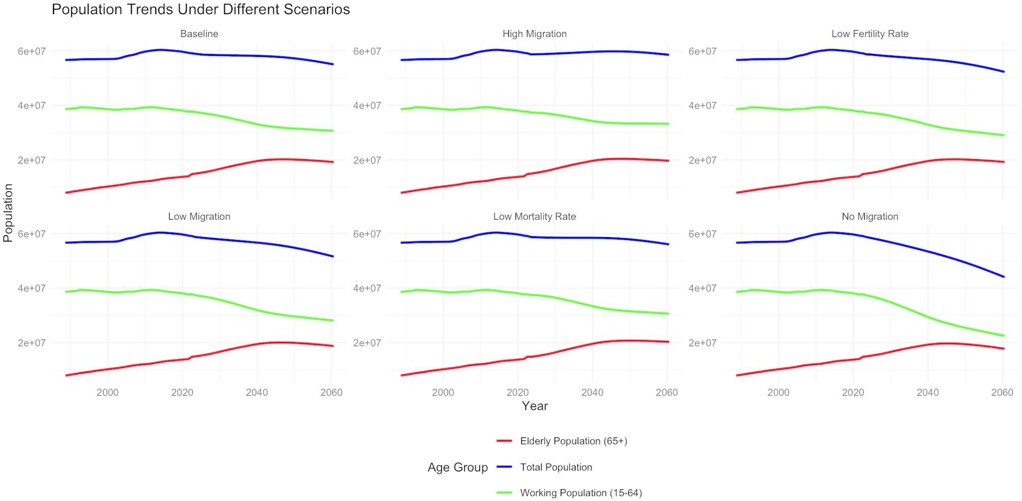
Population Projections: projections of the Italian population up to 2060 were sourced from Eurostat [25]. These projections were based on assumptions regarding future fertility, mortality, and migration rates, providing hypothetical scenarios for the population size and age structure.

GDP per capita served as an indirect indicator of per capita income, as its growth is considered a measure of economic development [26]. Healthcare expenditures per capita measured the consumption of healthcare goods and services, and social security expenses per capita acted as a proxy for public spending on social protection, primarily pensions (which are the most important social protection expenses in Italy) [27]. The ratios healthcare expenditure/GDP and social expenditure/GDP measured the share of resources used for healthcare or social security in relation to what is produced overall during the reference period.

The working population and population aged over 65 years were used to assess changes in the demographic structure, to better estimate shifts in economic and social dynamics in future years.

Because the Eurostat demographic paths are externally supplied, the resulting expenditure paths represent conditional projections. They should not be interpreted as probabilistic forecasts in the sense of an unconditional expectation but as ‘what‑if’ calculations contingent on the demographic assumptions [18].

All variables were log-transformed to normalize the data, reduce dimensional effects, and facilitate linearization, thereby enhancing the robustness and interpretability of the model. This transformation also helped address heteroscedasticity.

Bayesian vector autoregressive (BVAR) model

In recent decades, Vector Autoregressive (VAR) models have become standard tools in macroeconomic analysis and forecasting [28,29,30]. VAR models are favored for their simple formulation and effectiveness in capturing dynamic linear relationships between time series without imposing parameter restrictions. However, several issues arise when using the frequentist approach to estimate VAR models. For example, VAR models perform better with a small number of variables. Because of the limited number of unrestricted parameters that can be estimated, there is a risk of overfitting when too many variables are used. However, including only a few variables can result in omitted variable bias, leading to poor forecasting and structural analysis performance [30, 31]. Additionally, the VAR approach suffers from a loss of degrees of freedom with the extension of lag length, leading to large standard errors and unstable point estimates.

Since data for a limited period of time were available in our context, the BVAR approach offered significant advantages compared to VAR models [32,33,34,35,36,37,38,39]. Bayesian inference using parameter shrinkage, as described below, enhances the dynamic analysis and forecasting accuracy of models.

The BVAR approach combines sample information with researchers’ prior knowledge of the coefficients (priors) to derive a posterior distribution, thus incorporating additional knowledge during the estimation and achieving better results without the need for restricted models with many coefficients set to zero. The choice of prior is crucial; if the prior is too loose, overfitting is difficult to avoid, whereas if it is too tight, the data cannot sufficiently influence the results. Researchers usually set priors based on their understanding of the nature of the parameter or use informative priors to reflect their beliefs [32,33,34].

The specification of priors addresses two main issues: equations with too many free parameters tend to capture excess noise, and equations with too few parameters fail to adequately capture the signal. The use of priors provides a flexible solution for the trade-off between overfitting and signal extraction capabilities [37, 38].

Bayesian methods employ the maximum likelihood function to estimate posterior probabilities, overcoming the limitations of techniques such as the generalized method of moments (GMM) of Arellano and Bond (1991) [40]. This approach enhances the performance of structural estimation models (SEM), allowing for more accurate estimations [41].

We start with a standard Vector Autoregressive (VAR) model, represented as:

$$\: = \:c + \sum\nolimits_^p } + B + \:} $$

(1)

where p represents the maximum number of lags, c includes any constant terms, Yt is a vector of endogenous variables, Ai is matrices of coefficients, Xt is a vector of exogenous variables, B is the matrix of coefficients of exogenous variables and εt is the white noise error term with covariance matrix Σ [42].

When applying the Bayesian approach to VAR models, priors are combined with the likelihood function to derive a posterior distribution. The Litterman/Minnesota prior is particularly useful for the BVAR estimation. It assumes that the coefficients β are normally distributed with mean zero, expressing the a‑priori belief that, before observing the data, each lagged explanatory variable is expected to exert no effect on the current value of the dependent variable in every equation. For computational convenience the covariance matrix Σ is usually taken to be diagonal.

To mitigate the risk of overparameterization and ensure robust forecasting, we adopted a Litterman/Minnesota prior with conservative hyperparameters, carefully calibrated to balance the trade-off between overfitting and underfitting. Additionally, we restricted the lag length to one, based on minimization of the Bayesian Information Criterion (BIC) [43, 44].

Overall tightness (λ1)

controls the tightness of the prior distribution around the zero mean. A smaller λ1​ value implies a stronger influence of the prior (more shrinkage towards zero), whereas a larger λ1​ allows the data to be more influential.

Cross-variable lag decay (λ2)

adjusts the relative tightness for lags of different variables. For instance, it sets the prior variance for the lag of j-th variable in the i-th equation.

Exogenous variable tightness (λ3)

This regulates the tightness of exogenous variables, including the constant term.

Lag decay (λ4)

determines how prior variance decays with increasing lags. A value of λ4 = 1 implies a linear decay, whereas other values can specify harmonic or geometric decay.

Once the prior distribution is established, the posterior distribution of the parameters will also be normal, with the posterior mean and mode reflecting the information from both the prior and data.

The specification of the prior covariance matrix, ψ, influences the shrinkage applied to the parameter estimates, thereby defining the variability of the coefficients. The ψ matrix was determined using a two-step process. First, we utilized Autoregressive Integrated Moving Average (ARIMA) models to estimate the variance of the residuals for each variable. We utilised the R function `auto.arima()` (package forecast) to automatically select the best fitting ARIMA model based on the Akaike Information Criterion (AIC) [45], allowing us to identify appropriate lag structures and moving average components up to a maximum order of 2. This approach provided a preliminary assessment of the variability in each time series, and helped us set realistic priors that account for the data’s historical volatility and trend patterns. Then, the residual variances from the ARIMA models provided the basis for setting the elements of the ψ matrix.

In the Minnesota prior framework, the ψ matrix is often assumed to be diagonal, reducing the computational burden. This assumption implies that the variances of the error terms are independent across equations. The diagonal elements of ψ were set according to the residual variances estimated from the ARIMA models, ensuring that the prior variances reflected the inherent uncertainty in each variable’s historical data.

Therefore, we could ensure that the priors were neither too tight nor too loose, thereby striking a balance between preventing overfitting and allowing the data to adequately influence the posterior estimates based on observed data.

The BVAR model was estimated using the Metropolis-Hastings algorithm, a Markov‑chain Monte‑Carlo (MCMC) method that samples from the posterior distribution [46]. The posterior was sampled with the `bvar()` function from the *BVAR* package (version 1.0.5) in R. This routine implements an adaptive random‑walk Metropolis–Hastings algorithm. We ran four parallel chains of 15 000 draws each, discarding the first 5 000 as burn‑in (no thinning) and setting different random seeds via `set.seed()` for reproducibility. Proposal‑scale tuning followed the helper function `bv_mh()`. Convergence diagnostics, including trace plots and the Gelman-Rubin statistic, were used to ensure that the sampling process achieved convergence [47]. Convergence was assessed with the Gelman–Rubin potential‑scale‑reduction factor. This diagnostic runs several independent Markov‑chain Monte‑Carlo (MCMC) chains from deliberately over‑dispersed starting points and then compares how much the chains still disagree with one another (between‑chain variation) to how much each chain varies internally (within‑chain variation). When the chains have mixed well, these two sources of variation are nearly identical and falls close to 1 (we required R^ ≤ 1.05 for all parameters) [48].

Forecasting and scenario analysis

We conducted forecasts of the key economic indicators for each of the six demographic scenarios (Baseline, Low Mortality Rate, Low Fertility Rate, High Migration, Low Migration, and No Migration) up to the year 2060 [27]. These forecasts included healthcare expenditures per capita and social security expenses per capita, as well as ratio healthcare expenditures/GDP and social security expenditures/GDP. To incorporate demographic projections into the forecasting process, we used the Eurostat projections for the working and older populations as conditioning paths.

GDP per capita was treated as an exogenous variable, meaning it was not influenced by other variables that were treated as endogenous within the model. This decision was based on the rationale that GDP per capita, as a broad economic indicator, might be influenced by a wider range of factors not captured within our BVAR model’s scope. Consequently, we fixed the future projections of GDP per capita series during the estimation and forecasting phases: the best-fitting distribution was selected based on the highest R-squared value, ensuring the most accurate and reliable representation of the historical data’s characteristics. These projections were held constant as exogenous inputs in the BVAR model, ensuring that the influence of GDP per capita was consistent across all scenarios and not subject to the internal dynamics of the model.

By fixing GDP per capita, we provided a stable benchmark against which the impacts of healthcare and social security expenditures, as well as demographic changes, could be assessed. This methodology helped in understanding the direct consequences of demographic shifts on public finances without the confounding effects of fluctuating economic performance.

We computed Impulse Response Functions (IRFs) to examine the dynamic responses of the endogenous variables to shocks in the system. IRFs were calculated for a 38-year horizon to capture the long-term effects of demographic and economic changes on healthcare and social security expenditures. IRFs were calculated by rewriting the estimated BVAR in moving‑average form and then tracing what happens to each endogenous variable after a one‑standard‑deviation innovation to one of the other variables while all remaining shocks are held at zero [49].

Additionally, Forecast Error Variance Decompositions (FEVDs) were performed to determine the proportion of the forecast error variance of each variable that could be attributed to shocks from the other variables. The function fevd() takes those orthogonalised impulse responses and, for each horizon h, accumulates the squared contributions of shock k to the forecast error of variable j and divides by the total accumulated squared error, so that the shares add to 1 [50]. This helped in understanding the relative importance of each variable in driving the dynamics of the system.

The BVAR package provided both calculations directly through irf() (method irf.bvar) — that computes and stores impulse‑response functions and the associated forecast‑error‑variance decompositions and fevd() (method fevd.bvar), that returns a bvar_fevd object summarising the variance decompositions for each variable at each horizon.

Software and packages

The entire analysis was performed using the R programming language version 4.4.1 and RStudio version 2023.09.0 + 463; key packages BVAR, dplyr, ggplot2 were utilized. Forecasts were produced using the “predict” function in the BVAR package, specifying a 38-year horizon, until 2060. The forecasts were then exponentiated to revert the log transformation, making the results interpretable in their original units.