This study was conducted according to the Declaration of Helsinki and was approved by the Ethics Committee of the First Affiliated Hospital of Soochow University. Written informed consent was obtained from all subjects before their participation. Fifty-five patients with VM (47 females/8 males; age: 45.89 ± 12.29 years old; education level: 10.47 ± 4.79 years) and 57 demographically similar healthy controls (HCs) (48 females/9 males; age: 45.86 ± 12.37 years old; education level: 11.89 ± 4.77 years) were included in this study. The data presented here derived from our dataset collected between October 2020 and December 2022, and was partially overlapped with that employed in our previous publication on functional concordance [36]. In this study, the level of demographic factors between groups were matched to be as close as possible under the condition of sufficient and balanced sample sizes [37], and T1 structural images were utilized as the sole and principal image data. The diagnosis of VM were based on the criteria published by the Bárány Society and International Headache Society (ICHD-3 beta, appendix) [38, 39]. Videonystagmography, vestibular caloric test, video head impulse and audiometry tests were performed to rule out peripheral vestibular diseases. We collected demographic and clinical data from all patients using a standardized questionnaire, including sex, age, education level, migraine disease duration, vertigo disease duration, headache frequency (days per month), 10-point Visual Analog Scale (VAS), Dizziness Handicap Inventory (DHI), Migraine Disability Assessment Scale (MIDAS), Headache Impact Test-6 (HIT-6), Patient Health Questionnaire-9 (PHQ-9), and Generalized Anxiety Disorder-7 (GAD-7).

All patients with VM were not under regular preventive therapy and had not taken any therapeutic drugs within 3 days before MRI scanning. We performed MRI for patients with VM during the interictal stage. Patients were considered to be in the interictal period if they did not have vestibular or migraine symptoms at least 3 days before and 1 day after MRI acquisition. All the HCs had no history of migraine, vertigo, or any other types of primary headache. The following exclusion criteria were applied to all subjects: left-handedness; other neurological or psychiatric diseases; other pain conditions; drug or alcohol abuse; and MRI contraindications, such as pregnancy, claustrophobia, and ferromagnetic implants.

To determine whether the sample size was adequate in the current study, a power analysis was further conducted. Since there are no studies directly exploring the GM connectome in patients with VM, we reviewed previous literature of structural neuroimaging studies on VM (with a case-control design), and listed the effect sizes in Table S1. The minimum Cohen’s d in each research ranged from 1.02 to 1.47, which indicated extremely large effects, and we finally applied a conservative Cohen’s d of 0.80 (corresponding to a large effect). The G*Power software [40] was then used to estimate the required sample size with the following parameters: test family = t tests, statistical test = difference between two independent groups, tail(s) = two, effect size d = 0.80, significance criterion α = 0.05, and statistical power 1-β = 0.8. The required sample size was determined to be 26 for each group, indicating that our sample of 55 patients with VM and 57 HCs was adequate to provide sufficient statistical power for analyses.

All subjects were scanned using a 3.0-Tesla MRI system (MAGNETOM Skyra, Siemens Healthcare, Erlangen, Germany) with a 16-channel head and neck joint coil. Head motion and scanning noise were reduced by applying foam padding and earplugs. All subjects were instructed to lie still in the supine position with their eyes closed, relaxing and staying awake. High-resolution T1-weighted anatomic images were obtained using a sagittal fast spoiled gradient-recalled echo sequence: repetition time = 2300 ms, echo time = 2.98 ms, field of view = 256 × 256 mm2, matrix = 256 × 256, slice thickness = 1 mm, and slice number = 192. After the procedure, the images were immediately reviewed by two experienced radiologists to rule out visible lesions.

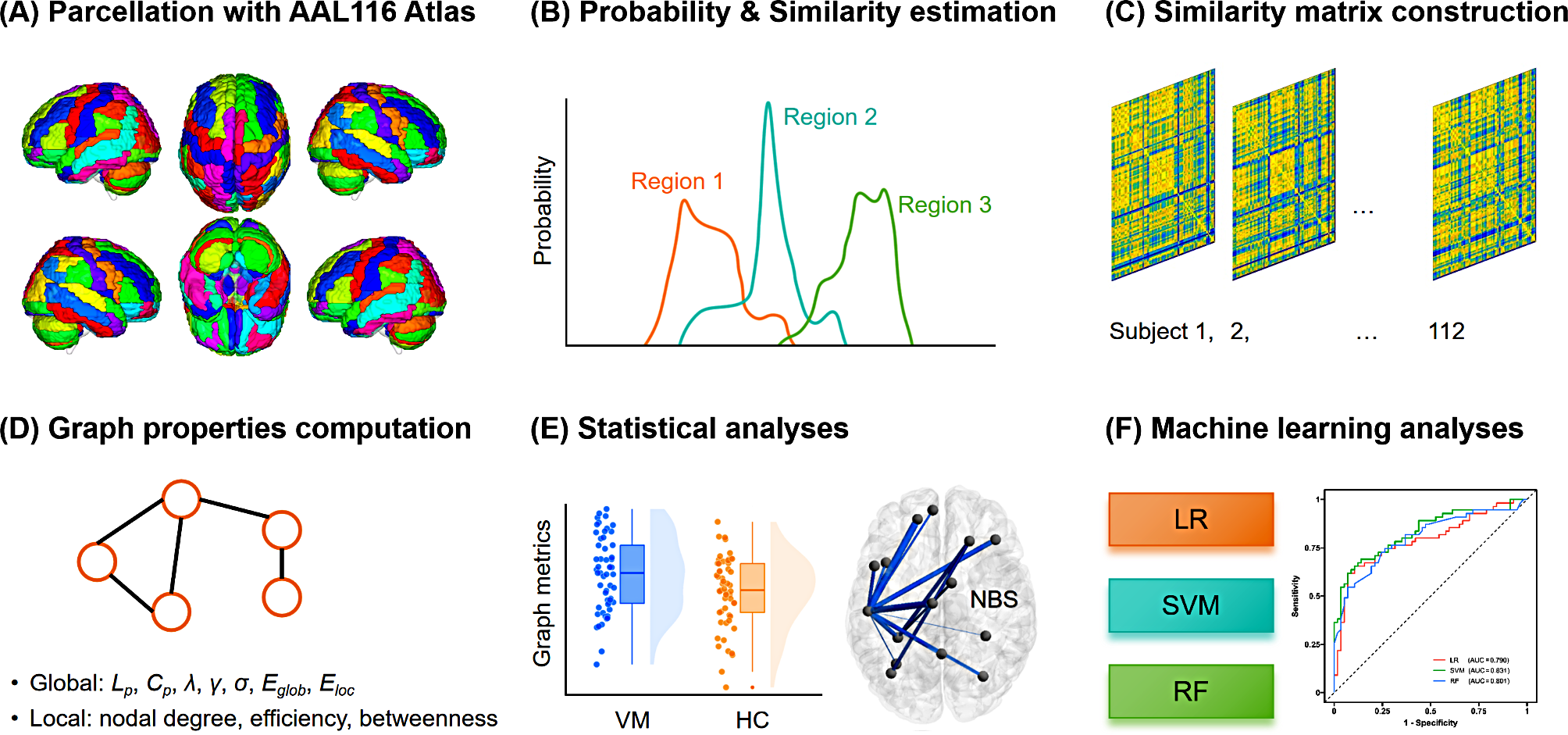
For structural MRI data processing, we used the Statistical Parametric Mapping analysis package (SPM12, http://www.fil.ion.ucl.ac.uk/spm/software/spm12/) along with the Computational Anatomy Toolbox for SPM (CAT12, http://www.neuro.uni-jena.de/cat/) for VBM analysis. In this procedure, all T1-weighted images were corrected for bias field inhomogeneities and then segmented into GM, white matter, and cerebrospinal fluid. The images were transformed into the standard Montreal Neurological Institute space by normalizing with a transformation integration of the diffeomorphic anatomic registration through exponentiated lie algebra algorithm and geodesic shooting, and resampled to 1.5 × 1.5 × 1.5 mm3. To preserve tissue volume after warping, voxel values in individual GM images were modulated by multiplying by Jacobian determinants derived from normalization. Finally, a GM volume map of each subject was created.

Based on the Automatic Anatomical Labeling atlas, the brain was divided into 116 regions of interest (ROIs), which served as nodes of the morphological brain network. Consistent with previous reports [32, 34], KL divergence was used to quantify the similarity of regional GM volume distribution between two regions (i.e., the edge between nodes), referred to as a morphological connection. To construct the GM morphological networks of each subject, we first extracted the GM volume values of all voxels within each ROI. The probability density function of these values was estimated using kernel density estimation with automatically estimated bandwidths, which was in turn used to compute the Probability Distribution Function (PDF) [41]. The KL divergence was then computed between two PDFs of each pair of ROIs. KL divergence quantifies the difference between two probability distributions, which equates to the information lost when a probability distribution is used to approximate another [42]. The standard KL divergence from the distribution Q to P is computed as follows:

$$}(P\parallel Q)\, = \,\sum\limits_^n \over },}$$

thus a 116 × 116 similarity matrix was generated for each subject by calculating the KLS values between all possible pairs of the 116 ROIs. However, because DKL(P‖Q) is unequal to DKL(Q‖P), we assessed the similarity between the two PDFs using a symmetric KL divergence, that is, DKL(P, Q) [31, 41], which is a derivate of the KL divergence and is calculated as follows:

$$}(P,Q)\, = \,\sum\limits_^n \over } + Q(i)\log \over }} \right)}.$$

Subsequently, the value of symmetric KL divergence was converted to a similarity measurement (range 0 [no similarity] to 1 [identical distributions]) for all pairwise regions using the following formula [31, 41]:

$$}P,Q)\, = \,}}}(P,Q)}},$$

and this produced 1 KLS-based SCN (116 × 116) for each subject, which was recognized as the final GM morphological network.

Network analyses were performed using the GRETNA toolbox (https://www.nitrc.org/projects/gretna/). To ensure that the morphological networks contained the same number of edges across participants at a fixed sparsity (i.e., the number of actual edges as a fraction of all possible edges), we used a sparsity-based thresholding procedure to convert them to a set of binary networks. A wide range of sparsity thresholds (0.05–0.30, with an interval of 0.01) [34] were used for binarization. In the resulting binarized SCNs, a value of 1 denotes significant covariation of the pairwise areas, and a value of 0 represents none.

Graph-theoretical properties were computed to quantify the topological characteristics of SCNs. For each individual morphological network at each sparsity level, we calculated global metrics including characteristic path length (Lp), clustering coefficient (Cp), normalized characteristic path length (λ), normalized clustering coefficient (γ), small-worldness (σ), global efficiency (Eglob), and local efficiency (Eloc). Herein, a set of random networks (number = 1000) were generated for the calculation of λ and γ. To characterize the network nodes, nodal metrics including nodal degree, nodal efficiency and nodal betweenness, were also computed. We further calculated the area under the curve (AUC) across the sparsity range (0.05–0.30, with an interval of 0.01) [34] as a comprehensive scalar measure of brain network topology for each metric, thereby avoiding potential bias of any single threshold.

Demographic and clinical data were analyzed using the SPSS software (version 27.0.1, IBM Corp., Armonk, NY, USA). For continuous variables, two-sample t-test (evaluating data with normal distribution) or the Mann–Whitney U test (evaluating data not normally distributed) was performed to compare differences between the VM group and HCs. The chi-square test was used to compare differences of categorical variables. The statistical significance threshold was set at P < 0.05.

The AUC of network metrics were compared between the VM group and HCs using an independent-sample t-test with sex, age, and education level as covariates of no interest in the GRETNA toolbox. For local topological characteristics, we used the false discovery rate (FDR) to correct for multiple comparisons at a significance level of P < 0.05.

The network-based statistics (NBS) method [43], implemented in the GRETNA toolbox, was used to localize specific pairs of regions with altered structural connections in the VM group. First, the edge-by-edge comparison of the strength of edge weight in the SCN matrix was performed between the VM group and HCs using the two-sample t-test. Second, the components that contained connected supra-threshold edges with P value of 0.001 were retained. Then, an empirical distribution of the connected component size was derived, and the largest component size was calculated by repeating the aforementioned steps with 5,000 permutations and setting the P value at 0.05 corrected for multiple comparisons. Before the permutation test, the potential confounding effects of sex, age, and education level were eliminated by multiple linear regression.

In the VM cohort, for network topological properties and connections that exhibited significant between-group differences, partial correlation analyses were performed to examine their relationships with clinical parameters, after controlling for the effects of sex, age, and education level. The correlation analyses were performed with SPSS 27.0.1, and the statistical threshold was set at P < 0.05.

To further validate the between-group differences of network topological properties and connections and to investigate their potential diagnostic value, three classifiers including LR, SVM, and RF were used to construct models for distinguishing individuals with VM from HCs. A combination of significant imaging features was used for the analyses. The nested cross-validation (CV) method was employed for machine learning, with 10-fold CV in the outer loop and stratified 5-fold CV in the inner loop. For the outer loop, min–max normalization was performed in each fold. For the inner loop, hyperparameter tuning was performed to optimize accuracy (LR and SVM: C = 2− 5, 2− 4, 2− 3, 2− 2, 2− 1, 1, 2, 4, 8, 16, and 32; RF: n_estimators = 10–200 with an interval of 10). After the completion of hyperparameter tuning in the inner loop, the optimal hyperparameters were used to train the final model based on the training set in the outer loop. Subsequently, model validation was performed with the testing set in the outer loop, yielding the accuracy, AUC, sensitivity, and specificity indices. Receiver operating characteristic (ROC) curve analysis was performed to examine classification performance. To validate the significance of accuracy and AUC, nonparametric permutation tests with 5,000 permutations were performed (statistical significance was set at P < 0.05). The mean weight (for LR and SVM) as well as the mean feature importance (for RF) across the CVs were employed as indicators of feature contribution to classification. We adopted the top 20% important features (sorted by absolute values of feature contributions) which simultaneously appeared in all models (LR, SVM, and RF) as the most contributed features for distinguishing individuals with VM from HCs.