The Medical Ethics Review Committee of the 1Amsterdam University Medical Centers (UMC) approved this study protocol and waived the need for informed consent. All patients were managed per institutional practices.

Datasets

This study retrospectively included four datasets comprising 1115 CTs from 931 patients with resectable, borderline resectable, locally advanced PDAC, and 195 CTs from 195 control patients. Table 1 outlines the characteristics of these datasets. The first dataset, REPDAC, represents the Amsterdam UMC and Leiden University Medical Center subset of the PREOPANC trials conducted by the Dutch Pancreatic Cancer Group [12, 13]. The second dataset, LAPC, includes patients from the Dutch Pancreatic Cancer Group LAPC registry [14]. The third dataset, CONTROL, comprises patients without pancreatic abnormalities who underwent CT scans before transcatheter aortic valve implantation. The fourth dataset, MSKCC, is a publicly available dataset from the Memorial Sloan Kettering Cancer Center [15]. We opted for late arterial phase CT scans (LAP-CTs) from the REPDAC, LAPC, and CONTROL datasets due to enhanced tumor and pancreas visibility at this phase, when available. However, for the MSKCC dataset, we utilized portal-venous phase scans (PVP-CT), as these were the only ones available, and two phases provide complementary information in PDAC segmentation [9]. All patients in the REPDAC, LAPC, and CONTROL datasets provided general informed consent.

Table 1 Dataset characteristics for the REPDAC, LAPC, CONTROL, and MSKCC datasetsData Preparation

One of three radiologists (C.Y.N, 27 years’ experience; F.S., 3 years’ experience; and M.K., 6 years’ experience) manually segmented the PDAC tumors in 256 LAP-CTs of 120 patients with (borderline) resectable PDAC (REPDAC dataset) and 66 LAP-CTs of 66 patients with LAPC (LAPC dataset) using a 3D slicer version 4.11.20210226 [16]. This manual segmentation was performed on the original unannotated CT scans to ensure precise delineation of tumor boundaries. In addition, to provide context and improve accuracy by enabling the model to distinguish PDAC from adjacent tissues more effectively, we independently automatically segmented surrounding anatomical structures, the pancreas, duodenum, spleen, kidneys, adrenal glands, liver, and gallbladder, using TotalSegmentator version 1.5.6 [17]. Figure S1 of the Supplement provides an example of a segmented LAP-CT.

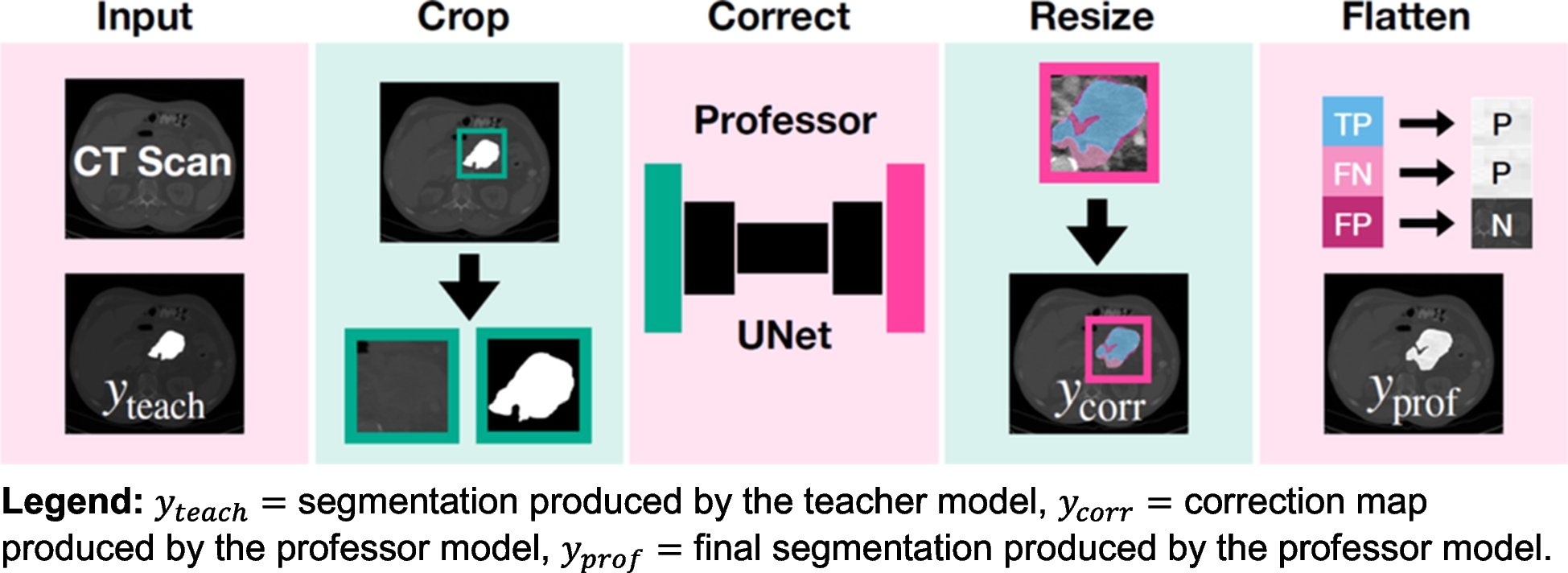
Model Implementation

We propose a professor model for automatically correcting pseudo-segmentations resulting from the teacher model as an addition to the conventional teacher–student framework in deep learning for medical image segmentation. The teacher–professor–student model extends the traditional teacher–student framework by introducing an intermediate refinement step. The professor model acts as a correction mechanism, improving the quality of pseudo-segmentations before they are used to train the student model, thus mitigating the propagation of errors in complex cases like LAPC. An overview of the proposed professor model is provided in Fig. 1.

Fig. 1

Architectural overview of the proposed professor model for PDAC segmentation refinement. The diagram illustrates the four sequential steps of the segmentation process: (A) initial segmentation by the teacher model (y_teach), (B) generation of the correction map (y_corr), (C) application of the correction matrix, and (D) production of the final refined segmentation (y_prof). This framework demonstrates how the professor model systematically improves upon the teacher model’s initial predictions through targeted correction mechanisms.

Preprocessing

To increase computational efficiency and reduce irrelevant contextual information, we first cropped the ground-truth and teacher-generated PDAC pseudo-segmentations and CT scans to a bounding box of the union of ground-truth and teacher-generated pseudo-segmentations.

Architecture

We used a 3D UNet model architecture for the professor model with an evenly weighted combination of DICE loss and cross-entropy loss and a fivefold cross-validation approach for training [18]. We employed a 3D U-Net architecture due to its ability to effectively capture volumetric spatial context, which is crucial for accurately segmenting the complex and infiltrative nature of pancreatic tumors [18]. We normalized the CT images according to their initial CT normalization applied during the teacher model’s training. The input for the professor model comprised the CT scans and the teacher-generated segmentations. The professor model’s training signals are derived from correction matrices denoted as ycorr, formulated using both the ground-truth ytrue and teacher-generated segmentations denoted as yteach. Specifically, we defined the professor model’s ground truthycorr as follows:

$$_=\left\ FN, if\ _\ne _\ and\ _=0\\ FP, if\ _\ne _\ and\ _=1\\ FN, if\ _=_\ and\ _=1\\ _, otherwise\end\right.$$

where yteach, ytrue = 1 for pixels belonging to the PDAC tumor, and yteach, ytrue = 0 for pixels belonging to the background according to the teacher model and ground truth segmentation, respectively. Here, FN represents false negatives, pixels incorrectly labeled as background but should have been identified as tumor, while FP denotes false positives, pixels erroneously marked as tumor that should have been classified as background. Conversely, TP identifies true positives, pixels accurately identified as tumor. These three categories are distinct, but the correction matrix allows for overlapping values for FN, FP, and TP, enabling various combinations and interpretations. This flexibility facilitates custom adjustments to prioritize specific error types.

We developed and tested four distinct correction matrices: Precision Priority, Pattern Discerner, Underestimation Focuser, and Inclusive Correction, each designed to address different error patterns. Precision Priority focuses on correctly identified tumor pixels (TP = 1), disregarding both types of misclassifications (FN = 0, FP = 0) under the assumption that errors lack systematic patterns for learning enhancement. Pattern Discerner addresses all prediction outcomes (FN = 1, FP = 2, TP = 3), assuming that the teacher model’s overestimations and underestimations exhibit identifiable, correctable patterns. Underestimation Focuser concentrates on correctly identified tumors and underestimations (FN = 1, TP = 2), intentionally omitting overestimations (FP = 0), based on the belief that underestimating tumor presence constitutes the most instructive error category for model refinement. Inclusive Correction focuses both on accurate tumor predictions and areas of overestimation (FN = 2, FP = 1, TP = 2), hypothesizing that the teacher model’s primary errors lie in overestimating tumor regions. A visual example of each correction matrix is provided in Fig. 2.

Fig. 2

Comparative visualization of correction matrices for LAPC segmentation refinement in arterial phase CT imaging. The figure presents ground-truth segmentations alongside teacher-generated predictions and demonstrates the four distinct correction matrix approaches: Precision Priority (emphasizing true positives), Pattern Discerner (weighted handling of FN = 1, FP = 2, TP = 3), Underestimation Focuser (prioritizing FN = 1, TP = 2), and Inclusive Correction (balanced approach with FN = 2, FP = 1, TP = 2). False negatives (FN), false positives (FP), and true positives (TP) are color-coded to illustrate the differing emphasis of each correction strategy. FN, false negatives; FP, false positives; TP, true positives

Resizing

We restored the correction matrix to the dimensions of the original segmentation.

Correction Matrix Transformation

We applied the predicted correction matrix to correct the teacher-generated segmentations as follows:

$$_=\left\1, if\ FN\\ 0, if\ FP\\ 1, if\ FP\\ _, otherwise.\end\right.$$

Model Training

The training was structured into three phases [1] training the teacher model on a small set of manually segmented data to segment PDAC, [2] training the professor model on a small set of manually segmented data to correct the teacher model’s segmentations, and [3] training the student model on the entire training set segmented by the teacher model and corrected by the professor model to segment PDAC. These steps are described in Fig. 3. This progressive approach allows each model to build upon the knowledge of its predecessors while maintaining specialization in their respective tasks. While this approach incorporates elements of self-supervised learning, particularly in the teacher–student framework, it also shares characteristics with semi-supervised methods. The initial training of the teacher model on manually labeled data, followed by the use of unlabeled data for the student model, aligns more closely with semi-supervised paradigms. However, the introduction of the professor model for refining pseudo-labels introduces a self-supervised component. This hybrid approach leverages the strengths of both methodologies: the ability to learn from limited labeled data (semi-supervised) and the capacity to improve representations without additional human annotation (self-supervised).

Fig. 3

Comprehensive workflow diagram of the enhanced self-supervised learning framework for PDAC segmentation. The schematic details the three-phase training process: (1) teacher model training on manually segmented data, (2) professor model training for segmentation refinement, and (3) student model training using the refined segmentations. This diagram illustrates the novel integration of semi-supervised and self-supervised learning approaches, highlighting the unique role of the professor model in improving segmentation quality

The Teacher Model

Training consisted of 517 CTs described in Table 2 with manual segmentations of the PDAC tumor if present and automatic segmentations of surrounding anatomical structures obtained from TotalSegmentator [17]. The teacher model comprised a simple nnUNet architecture involving a two-stage 3D UNet cascade [19]. The initial UNet in this setup was trained on downsampled images to create low-resolution segmentations. These low-resolution outputs were then used as additional inputs for training the full-resolution UNet. The low-resolution stage processed inputs at approximately 2.85 × 1.45 × 1.45 mm spacing with patch sizes of 96 × 160 × 160 voxels, while the full-resolution stage operated at 2.0 × 0.71 × 0.71 mm spacing with patch sizes of 64 × 192 × 160 voxels. Both stages utilized a base feature count of 32 channels in the initial layer, increasing to a maximum of 320 channels in the deepest layers. The network architecture consisted of six encoder stages and five decoder stages, with two convolutional layers per stage (3 × 3 × 3 kernels). The downsampling path employed pooling operations with varying strides across different axes, optimized for the anisotropic resolution of CT scans.

Table 2 Training sets for the Teacher, Professor, and Student modelsThe Professor Model

Training consisted of 106 CTs described in Table 2 with PDAC segmentations generated by the teacher model during the teacher model’s cross-validation across five training folds. We excluded the CONTROL scans as these do not contain a tumor and reduced the number of REPDAC scans to focus on LAPC specifically. The professor model used a standard UNet architecture, operating at a spacing of 2.0 × 0.70 × 0.70 mm with patch sizes of 24 × 64 × 80 voxels. This model processed both the original CT data and the teacher’s predictions as dual-channel input (CT intensities and segmentation masks). The network consisted of five encoder stages and four decoder stages with two convolutional layers per stage, using 3 × 3 × 3 kernels. The professor model employed asymmetric pooling strategies with two pooling operations along the z-axis and four pooling operations along the x and y axes. The specific pooling kernel sizes were [1, 1, 1], [1, 2, 2], [2, 2, 2], [2, 2, 2], and [1, 2, 2] for the five stages, preserving z-axis resolution in the first, second, and final pooling stages. We selected the correction matrix of the best-performing professor model for segmenting LAPC during the fivefold cross-validation.

The Student Model

Training consisted of 1085 CTs from 903 patients described in Table 2. First, we used the teacher model to segment 568 CTs of this dataset for which no manual segmentations were available. Second, we used the professor model to correct these PDAC segmentations. Finally, we trained the student model with the resulting teacher-segmented and professor-corrected CTs and the manually segmented 517 CTs used to train the teacher model. We employed the same 3D UNet cascade network architecture for the student and teacher model, with slight differences in configuration parameters. The low-resolution stage operated at 2.53 × 1.30 × 1.30 mm spacing with patch sizes of 64 × 192 × 192 voxels, while the full-resolution stage processed inputs at 2.0 × 0.76 × 0.76 mm with patch sizes of 48 × 192 × 192 voxels. The student model maintained the same network design principles, with six encoder stages, five decoder stages, 32 base features increasing to 320 maximum features, and identical convolution kernel sizes.

Training Hyperparameters

All models were trained using the SGD optimizer (momentum = 0.99, nesterov = true, weight_decay = 3e−5) with an initial learning rate of 0.01 and polynomial decay. We employed a fivefold cross-validation approach using a combined Dice and cross-entropy loss function with deep supervision. Training continued for 1000 epochs with 250 iterations per epoch, and validation was performed every 50 iterations. The data augmentation pipeline included spatial transformations (rotations ± 30°, scaling 0.7–1.4), Gaussian noise, Gaussian blur, brightness and contrast adjustments, and mirroring along all axes. We used a batch size of 2 for the teacher and student models and 3 for the professor model, constrained by GPU memory.

Performance Evaluation

We used multiple metrics to comprehensively evaluate segmentation performance. The Dice Similarity Coefficient (DSC) measured overall segmentation accuracy through volumetric overlap. To assess boundary accuracy, we calculated Hausdorff Distance 95 (HD95), which quantifies the 95 th percentile of the maximum surface distance between segmentations, and Mean Surface Distance (MSD), which measures the average minimum distance between segmentation surfaces. Additionally, we computed sensitivity (proportion of actual tumor voxels correctly identified) and specificity (proportion of non-tumor voxels correctly identified) to evaluate the models’ clinical utility in detecting tumors and sparing healthy tissue.

We evaluated all three models on a test dataset containing 30 randomly selected CTs from 27 patients from the LAPC dataset that were not used to train the teacher, professor, or student segmentation model. To address patient-level correlation in our dataset, we ensured all scans from the same patient were assigned to a single partition (training or testing). We applied a Wilcoxon signed-rank test to assess the statistical significance of performance differences between teacher-generated and professor-corrected segmentations across all metrics. A p-value of 0.05 was considered statistically significant.