Patient Cohort

SIRT with personalized dosimetry was conducted for 28 patients with different types of liver cancers, utilizing 90Y bremsstrahlung SPECT/CT imaging, at Geneva University Hospital, Switzerland, between November 2021 and January 2023. This retrospective study was approved by the institutional ethics committee and the requirement to obtain informed consent was waived. Among this number of patients, 17 were treated for hepatocellular carcinoma (HCC) tumors and were included in this retrospective study. Glass microspheres (Therasphere™; Boston scientific group, Marlborough, Massachusetts) were used for treatment. Selection criteria for SIRT included: Adult patients with at least one well-defined tumor > 3 cm, stable liver enzymes, no contraindications to angiography, no concurrent treatment, no previous transplantation, or previous liver resection and an Eastern Cooperative Oncology Group (ECOG) performance status of 0 to 1. Patient characteristics are summarized in Supplemental Table 1. The Mann–Whitney U test and Fisher’s Exact test were used to compare the clinical continuous and categorical features between responder and non-responder groups, respectively.

90Y-SIRT Treatment

After mapping the liver vessels and evaluating the extrahepatic shunts, personalized voxel-level dosimetry and treatment planning were performed using 99mTc-MAA SPECT/CT imaging for each patient to simulate the therapy. Lung shunt fraction (LSF) was calculated based on planar images. Post-treatment absorbed dose distributions were calculated through 90Y bremsstrahlung SPECT/CT imaging. Simpliciti90Y™ (Mirada Medical Ltd, United Kingdom) treatment planning system was used for dosimetry calculations. The median of 99mTc-MAA injected activity was 156 ± 9.7 MBq, whereas the median of 90Y injected activity was 2.8 ± 1.17 GBq. The initial activity was calculated using the partition model specified for each individual.

Image Analysis

Baseline diagnostic images were acquired either by multi-phasic contrast-enhanced CT (Siemens Healthineers, SOMATOM, Erlangen, Germany) at 100 kVp and the tube current of 315.2 ± 216.71 mA (average ± SD), or 3T MRI (Siemens healthineers, Erlangen, Germany). SPECT/CT images were acquired on a dual-head Symbia-T series camera (Siemens Healthineers, Erlangen, Germany) using a low-energy high-resolution collimator. The energy window center of 99mTc SPECT was set to 140 keV [128–150]. A matrix size of 128 × 128, with 128 views, over a 360-degree arc and 20–25 s per view were utilized. The bremsstrahlung SPECT/CT scans were acquired under a continuous energy window [105–195] keV using high energy collimators, and 128 frame with 15–30 s per frame. SPECT/CT data were reconstructed using a 3D ordered-subset expectation maximization (3D-OSEM) algorithm with 4 iterations and 8 subsets. Reconstruction was performed with attenuation correction but without scatter correction followed by 5mm Gaussian post-reconstruction filtering.

The follow-up (FU) contrast-enhanced CT was acquired on SOMATOM scanner (Siemens Healthineers, Erlangen, Germany) 1 month and every 3 months post-therapy mostly with 100 and 120 kVp and 352.14 ± 135 mA (average ± SD) tube current. If CT images at a specific timepoint were not acquired, 3T MR images (Siemens healthineers, Erlangen, Germany) were collected. Tumor boundaries were localized, and target volumes (tumors) delineated on arterial phase of baseline and FU images by an experienced nuclear medicine physician and gastrointestinal (GI) interventional radiologists who were blinded to clinical, biological, survival, and dosimetry data. To assess the outcome, tumor response was evaluated up until 3 months post-treatment based on modified response evaluation criteria in solid tumors (mRECIST) comparing relative changes in tumor largest diameter on axial view of CT or MRI (if CT was unavailable) [18]. Based on the response to treatment, patients were categorized as responders (R) (including complete response [CR] meaning disappearance of any intertumoral arterial enhancement in all target lesions, and partial response [PR] groups meaning at least a 30% decrease in the sum of the diameters) and non-responders (NR) (including stable disease [StD] meaning insufficient shrinkage to qualify for PR and insufficient increase to qualify for progressive disease [PD], and PD groups, meaning an increase of at least 20% in the sum of the diameters of viable target lesions) by GI interventional radiologists.

Dosimetry Calculations

After tumor manual delineation by a nuclear medicine physician on diagnostic images, tumor segmentations were transferred onto SPECT/CT images by registration of diagnostic images and co-registered CT of SPECT/CTs performed using elastix library and a two-step rigid and deformable registration using mutual information similarity metric [19]. The registration step was performed using rigid-body registration followed by deformable algorithms. The perfused lobe and whole liver were delineated on the co-registered ACCT of SPECT/CT images by a physician and a previously trained deep learning model [20], respectively. Normal structures namely, normal perfused liver (NPL) and whole normal liver (WNL) were obtained by subtracting the tumor from the perfused lobe and whole liver.

The physical as well as the biologically effective dose (BED) distributions were calculated for both 99mTc and 90Y SPECT of each patient. An in-house MATLAB code (MATLAB (2022b), Natick, Massachusetts: MathWorks Inc) was validated against replicated analysis with Simplicit90Y™ (Boston Scientific, Marlborough, MA) and was utilized to calculate the 3D voxel-level physical dose maps based on local energy deposition method. 3D voxel-level BED maps were also calculated for tumoral and normal structures separately using the following formula:

$$BED=D\left(1+\frac^\!\left/ \!_\right.} . \frac_}_+_}\right)$$

(1)

where D is the cumulative dose of 90Y radiation, TRep is the sublethal damage repair half-time and Tphys is the radionuclide decay half-life (64.2 h). α⁄β ratios and TRep for Tumor and normal tissue are derived from Chiesa et al. study [21]. The designated values for α⁄β were 10, while TRep (h) was set to 1.5 and 2.5 for Tumoral and Normal structures, respectively. The DVC parameters extracted from 99mTc and 90Y DVHs and biologically effective dose-volume histograms (BVHs) for each structure are listed as follows:

The evaluated parameters include the volume of structures, mean absorbed dose, maximum dose, minimum dose, D50, D70, D95, D98, V120, V205, and V400 for all structures. Additionally, for NPL and WNL, V20, V30, V50, V70, and V90 were also assessed. All volume-based constraints (V20-V400) were calculated using both milliliter (ml) and percentage (%) units.

Additionally, we computed other features, such as a simplified version of the tumor dose homogeneity index (HI = D5/D95), commonly used in external beam radiotherapy (EBRT). Furthermore, we calculated the tumor to normal liver ratio (TNR) with respect to both NPL (TNRNPL) and WNL (TNRWNL) for both 99mTc and 90Y procedures. Two other (personalized) dosimetry-related parameters, including LSF, and 90Y-injected activity were also utilized as predictive features. A Mann–Whitney U-test was conducted to compare the dose values between the R and NR groups.

Radiomic and Dosiomic Feature Extraction

The radiomic features were extracted from co-registered CTAC and SPECT images while dose maps, whether physical or BED maps, were utilized for extracting dosiomic features. CT images were resampled to 1.5 × 1.5 × 1.5 mm3 and clipped between −500 to 500 HU prior to feature extraction. SPECT images were clipped between 0 and 99.9th percentile of the counts/s values for each image. Dose maps were clipped within the range of 0 to the median of 95th percentile of the dose values (Gy) across all patients, varying based on the anatomical structure and radionuclide used, i.e., fixed values were used for all patients. For 99mTc dose maps, these values were 650.34, 158.02, and 127.08 Gy for the tumor, NPL and WNL, respectively. Similarly, for 90Y dose maps, the corresponding values were found to be 416.25, 133.16, and 123.08 Gy for the tumor, NPL and WNL, respectively. For extracting the features, the bin width was set to 50 counts/s, 20 HU, and 1 Gy for SPECT, CT, and dose maps, respectively. These bin width values were selected to make a compromise between keeping the valuable information and computational effort. For example, the bin width of the dose maps was selected to be 1 Gy to keep the details of dosimetry calculations while maintaining an efficient computational burden and time.

A total of 321 features were calculated for all three structures (tumor, NPL and WNL), comprising 107 features each, using pyradiomics library (version 3.1.0) [22]. Each set of features consists of 19 First-Order Statistics, 16 Shape-based (3D), 10 Shape-based (2D), 24 Gray Level Co-occurrence Matrix, 16 Gray Level Run Length Matrix, 16 Gray Level Size Zone Matrix, 5 Neighboring Gray Tone Difference Matrix, and 14 Gray Level Dependence Matrix features. The features for all structures were combined and used in the next steps.

Strategy Devising

We devised multiple strategies to comprehensively evaluate all potential scenarios:

1)

Radiomics from 99mTc MAA SPECT or CT images,

2)

Radiomics from 90Y SPECT or CT images,

3)

Dosiomics from MAA physical or BED dose maps,

4)

Dosiomics from 90Y physical or BED dose maps,

5)

DVH-driven parameters from MAA dose maps,

6)

DVH-driven parameters from 90Y dose maps.

Each of these six categories encompasses six subcategories, including:

DVH and Dosiomics a)

Physical dose denoted as “Dose”

b)

BED

c)

Dose + BED

d)

Dose + Clinical

e)

BED + Clinical

f)

BED + Dose + Clinical

Radiomics a)

CT

b)

SPECT

c)

CT + Clinical

d)

SPECT + Clinical

e)

CT + SPECT

f)

CT + SPECT + Clinical

This results in a total of 36 different strategies. In addition, 16 clinical features were used which are indicated in Supplemental Table 1, among them sex and extrahepatic metastasis (only one patient had metastasis) were not used because of extreme unbalance between R and NR groups. A Mann–Whitney U-test was also conducted to compare the radiomics and dosiomics feature values between the R and NR groups. The test was followed by a Benjamini and Hochberg (BH) test with q = 0.05 to adjust the p-values and find the false discovery rate.

Feature Selection and Machine Learning Modeling

To train the models, we employed a threefold nested cross-validation (CV) approach, comprising an inner and an outer CV loop, to prevent overfitting and ensure a more reliable performance. Features extracted from training sets of each strategy were normalized to their Z-score, with the resulting mean and standard deviation applied to corresponding features extracted from the test datasets within the outer loop.

Different machine learning (ML) algorithms combined with different feature selection (FS) methods, aiming at identifying the most relevant features and eliminating redundant ones, were utilized. ML modeling was carried out using eight different algorithms, including Decision Tree (DT), Generalized Linear Mixed Model Boosting (GLMB), Logistic Regression (LR), Multiple Layer Perceptron (MLP), Naïve Bayes (NB), Random Forest (RF), Support Vector Machine (SVM), and Extreme Gradient Boosting (XGB). We used five different FS methods, including ANOVA, Kruskal, Minimum Redundancy Maximum Relevant (MRMR), Randomized Ensemble Feature Importance (Relief), and Recursive Feature Elimination (RFE). The redundant features were removed using Spearman's rank correlation coefficient. A rho of 0.90 was used as threshold.

Hyperparameter optimization was carried out using Grid Search with threefold cross-validation within the inner CV loop, and the best values employed for model training. Given the small sample size, we also generated 1000 bootstrap samples with replacement for ROC curves. The dataset was imbalanced between the number of treatment non-responders and responders. Synthetic Minority Oversampling Technique (SMOTE) was used on the training sets to overcome any biases in model performance due to unbalanced dataset. SMOTE was used during hyperparameter optimization on the inner training dataset, and once the best hyperparameters were chosen, it was also applied to the outer training dataset. The final trained model was evaluated on the outer test dataset. Eventually, we ended up trying 1440 models (resulting from 8 ML × 5 FS × 6 categories × 6 subcategories). Supplemental Table 2 summarizes the hyperparameters and their ranges for each classifier.

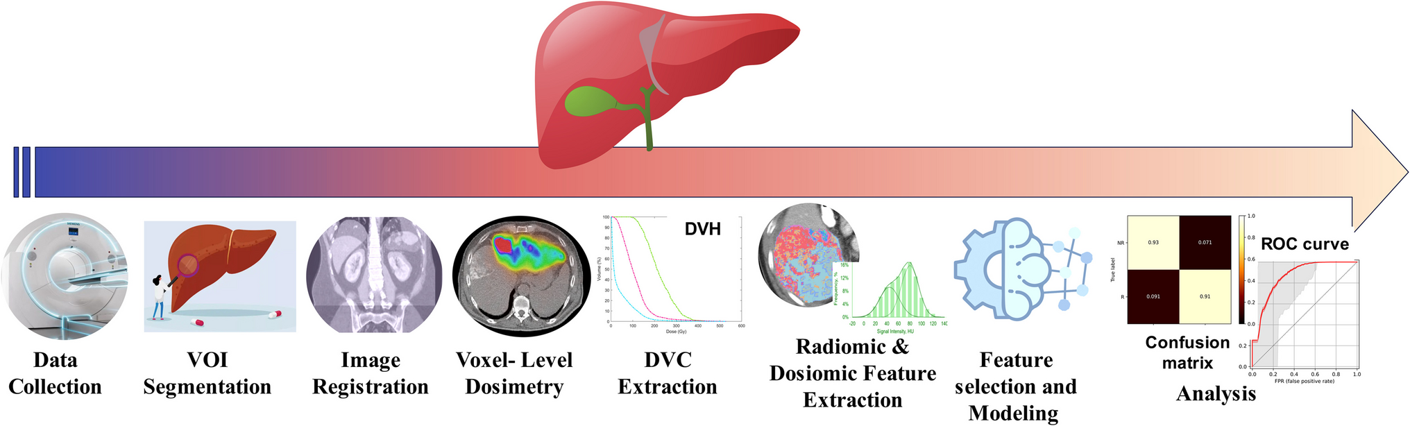
For every model, a confusion matrix was computed, detailing true negative (TN), true positive (TP), false negative (FN), and false positive (FP) rates. Model performance was assessed using metrics, such as Area Under the Receiver Operating Characteristic Curve (AUC), accuracy (ACC), sensitivity (SEN), and specificity (SPE). To ascertain the most robust models, Delong statistical test was employed to compare AUC values, with a P-value < 0.05 indicating statistical significance. Figure 1 outlines the study's flowchart whereas Fig. 2 summarizes the machine learning procedure.

Fig. 1

Flowchart depicting the procedural steps followed in this study. VOI: volume of interest, DVC: dose-volume constraint

Fig. 2

The machine-learning procedure and 3-fold nested cross-validation concept. After feature extraction and normalization, five different feature selection methods were used to eliminate the redundant features. The selected features were used for machine-learning procedures with eight different algorithms in a 3-fold nested cross validation framework. The AUC, Accuracy (ACC), Specifity (SPE) and sensitivity (SEN) were calculated