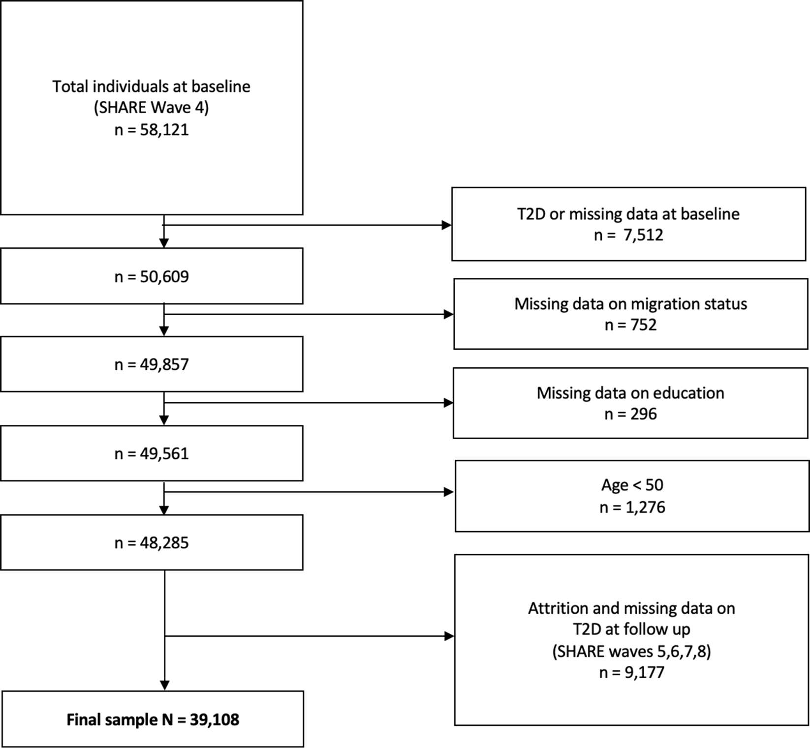
We used data from SHARE, which is the largest pan-European social science panel study, providing cross-disciplinary longitudinal data on demographic, socioeconomic, and health variables for people aged 50 years or older and their coresidential partners (16). SHARE data are collected biannually through computer-assisted personal face-to-face interviews (CAPI), and the survey has been extensively described elsewhere [23]. The SHARE questionnaires were revised and modified from Wave 4 onwards [24], meaning that some measures cannot be directly compared with those from Waves (1–3). Hence, we used Wave 4 (2011) as the baseline. We then followed individuals over all subsequent Waves that were available at the time of analysis (i.e., Waves 5, 6, 7, and 8 conducted in 2013, 2015, 2016, and 2019–2020, respectively), resulting in a follow-up period of approximately 9 years (2011–2020). All SHARE respondents aged 50 years and older, without known T2D or other diabetes diagnosis in Wave 4, and without missing data on social strata variables at baseline were included in the analysis (Fig. 1). The initial sample comprised 58,121 individualsFootnote 1, of whom 7,197 (12.4%) already had an existing T2D diagnosis at baseline (see Supplementary Table S1 for characteristics of individuals with existing T2D at baseline). To examine the longitudinal onset of T2D, only respondents without T2D at baseline and with available data at follow-up were included in the analysis. In order to minimize the number of observations lost to follow-up, we included respondents with available data on presence of T2D on any of the follow-up Waves [10]. The final analysis sample consisted of N = 39,108 respondents who were at risk of developing T2D. In case of conflicting information on consecutive follow-up Waves (i.e., a present diagnosis recorded for an intermediate Wave but not for the following consecutive Wave), the presence of self-reported diabetes on any Wave was coded as onset of T2D. Conflicting information was found for n = 1,020 cases (28% of those with T2D).

The SHARE unique participant identifier was used to link observations from the same participant across survey Waves. Figure 1 provides an overview of study population flow. SHARE was granted ethics approval by the Ethics Council of the Max-Planck-Society.

Study population flowchart

Based on the question “Has a doctor ever told you that you had any diabetes or high blood sugar?” in follow-up Waves 5, 6, 7 and 8, the dichotomous outcome variable onset of T2D (0 = no onset of T2D; 1 = onset of T2D) was computed for all respondents at follow-up.

We generated 72 (= 2 × 2 × 2 × 3 × 3) intersectional strata based on the combinations of sex/gender (2 levels), migration background (2 levels), living arrangement (2 levels), education level (3 levels) and household income (3 levels): sex/gender, migration background, living arrangement, education level and household income. These categories were chosen based on known social determinants of T2D [25]. Sex/gender was coded as male or female. Migration background was defined by country of birth: those who were born in their current country of residence were categorized as non-migrants, those who were born in a different country were categorized as migrants. Living arrangement was defined dichotomously as living alone or sharing a household with at least one other person such as a spouse, partner or other family member. Education level was classified according to the International Standard Classification of Education (ISCED 1997) and coded into three categories: high (ISECD 1997 level 5–6), mid-level (ISECD 1997 level 3–4) or low education (ISECD 1997 level 0–2). Finally, tertile values of the SHARE household income variable were used to categorize household income as highest income group, medium income group or lowest income group. We calculated the tertile values based on the data available for the total sample in SHARE Wave 4. The household income was either directly reported by respondents, or in cases of missing data, one of the available multiple imputations in SHARE was used, according to the methodology described elsewhere [26]. We adjusted the income that was provided in national currencies in the data by purchasing power parity (PPP) exchange rates in order to allow cross-sectional country comparisons of financial variables, with Germany as a reference country. As not all respondents in Wave 4 were selected in our final sample (i.e., due to missing data), the tertile values do not reflect equal thirds of the sample but rather correspond to the actual income position within the interview country. Overall, n = 13,539 (34,6%) of the final sample were assigned to the highest income group, n = 13,015 (33,3%) were assigned to the medium income group and n = 12,554 (32,1%) were assigned to the lowest income group.

We performed an I-MAIHDA for the onset of T2D with individual respondents (level 1) nested in social strata (level 2). Following the procedure developed by Evans and Merlo [13, 15, 16, 27], the onset of T2D was analysed through three successive multilevel logistic regression models described below. We also calculated the AUC as a well-established measure of discriminatory accuracy in clinical epidemiology [28]. All analyses were run in Stata/BE®18.0 (Statacorp, College Station, TX, USA). P-values < 0.05 (two-tailed) were considered statistically significant.

In a first step, the simple intersectional model included only an intercept and random effect for the social strata (null model). This model provides information on the overall inequality in the sample by producing stratum-specific predictions of T2D onset and summarizing the degree of heterogeneity within and between strata. The outcome predicted onset of T2D and 95% confidence intervals (95%CI) were estimated for each of the 72 social strata based on model 1. No covariates were included in the null model as it was used to conduct a simple analysis of the individual variance components (i.e., between and within-strata variance) and to compute the Variance Partition Coefficient (VPC), often also referred to as the Intraclass Correlation Coeffcient (ICC). The VPC provides an estimate of the variance in T2D onset that lies between strata. A higher VPC indicates a higher degree of clustering of T2D onset within strata, i.e., greater similarity in T2D onset within the strata and greater differences across the strata. The proportion of T2D variation that lies within the strata is indicated by 1-VPC.

A challenge in estimating the VPC in multilevel logistic regression is that, in contrast to multilevel linear regression with continuous outcomes, the level-1 (i.e., respondent-level residuals) cannot be estimated directly. We adopt the widely used approach based on the latent response formulation of the model and estimate the VPC as follows [29]:

$$\:VPC=\:\frac_\end}^}_^+3.29\end}\:\times\:\:100$$

,

where multiplication by 100 allows for interpretation in percentage terms. In this equation, \(\:_\end}^\)denotes the between-stratum variance in the onset of T2D, while 3.29 denotes the within-strata between-individual variance constrained equal to the variance of the standard logistic distribution [29]. This model was also intended to determine the predicted T2D onset for each of the intersectional strata. Since the probability scale favours interpretation, the predicted logit (log-odds) of developing T2D were transformed into the probability of developing T2D for every intersectional stratum [30].

As recently pointed out by Axelsson Fisk and colleagues [30], there is no unified classification system for interpretation of VPC values in social epidemiology. However, based on the widely accepted grading of Intraclass Coefficients (ICC), the authors propose the following classification of discriminatory accuracy: non-existent (0–1), poor (> 1 to ≤ 5), fair (> 5 to ≤ 10), good (> 10 to ≤ 20), very good (> 20 to ≤ 30), excellent (> 30).

In the main effects model, all social strata variables are included additively (sex/gender, migration background, living arrangement, education level and household income) as fixed effects. Odds ratios (ORs) and 95%CI were also estimated for the strata variables (i.e. sex/gender, migration background, living arrangement, education level and household income), with ORs above 1 indicating an increased chance of developing T2D at follow-up whereas ORs below 0 indicate a reduced chance. The Proportional Change in Variance (PCV) was calculated to quantify the proportion of the stratum-level variance from the unadjusted intersectional model that is explained by the additive main effects. The PCV was calculated as:

$$\:PCV=\:\frac\begin\begin_^-\:_^\end\end\end}_^}\:\times\:\:100$$

In the PCV equation, \(\:_^\) and \(\:_^\) denote the between stratum variance derived from models 1 and 2. The PCV was multiplied by 100 to obtain percentages. A high PCV indicates that most of the stratum-level variance is explained by the additive main effects, while a low PCV indicates that it is explained by multiplicative between-strata interactions, i.e., by intersectional effects [31]. Furthermore, we obtained estimates of stratum random effects to measure stratum-specific risk and identify strata with higher and lower T2D risk than expected based on the additive main effects only. This is done by decomposing the absolute risk of T2D into two parts: (1) risk of T2D explained by the main effects and (2) risk of T2D explained by higher order interaction effects between the included variables. The random effects (interactions) of each stratum allow us to assess the presence and magnitude of such stratum-specific hazardous or protective interaction effects [19]. For the purpose of a sensitivity analysis, we calculated an additional intersectional model including all the social strata variables and adjusted for age and country. The PCV and estimates of T2D risk at the stratum-level based on model 3 are provided in the supplementary material (supplementary Tables S2 and S3).