2.1 Study Populations and Clinical Data

This popPK analysis included data from seven phase I and phase II studies; four in healthy participants (studies ARRAY-380-103, ONT-380-012 [NCT03723395] [9], SGNTUC-015 [NCT03914755] [10], and SGNTUC-020 [NCT03826602] [11]), one in patients with HER2+ mCRC (study SGNTUC-017 [NCT03043313] [4]), and two in patients with HER2+ mBC (studies ONT-380-004 [NCT01983501] [12] and ONT-380-005 [NCT02025192]) (Table S1 of the Electronic Supplementary Material (ESM)). All studies were conducted in accordance with the Declaration of Helsinki and the International Conference of Harmonization Guideline for Good Clinical Practice. All studies were approved by an institutional review board or ethics committee at each site. All participants provided written informed consent for study-related treatments and procedures.

Data from HER2CLIMB (ONT-380-206) were not included in the popPK model development as time from the dose prior to the PK samples was not recorded, preventing determination of the time of the PK sample collection after the preceding dose. Data from the healthy participant studies only included tucatinib PK data from those administered the currently marketed tablet formulation in the fasted state. Population pharmacokinetic evaluable participants had received at least one tucatinib dose and had at least one measurable tucatinib concentration that included dose and sampling time information. ARRAY-380-103 was a study conducted in healthy participants to evaluate tucatinib PK following a 300-mg single PO dose comparing fasted and fed states, in combination with omeprazole and with a previous formulation (powder-in-capsule, not the approved formulation) [6]. ONT-380-012 was a drug–drug interaction study conducted in healthy participants evaluating tucatinib (300 mg PO single dose or BID) as a victim and perpetrator [9]. SGNTUC-015 was a study evaluating the PK of tucatinib between Caucasian and Japanese subjects at 50, 150, and 300 mg PO BID [10]. SGNTUC-020 was a study evaluating the impact of tucatinib (300 mg BID) as a perpetrator on metformin PK in healthy volunteers [11].

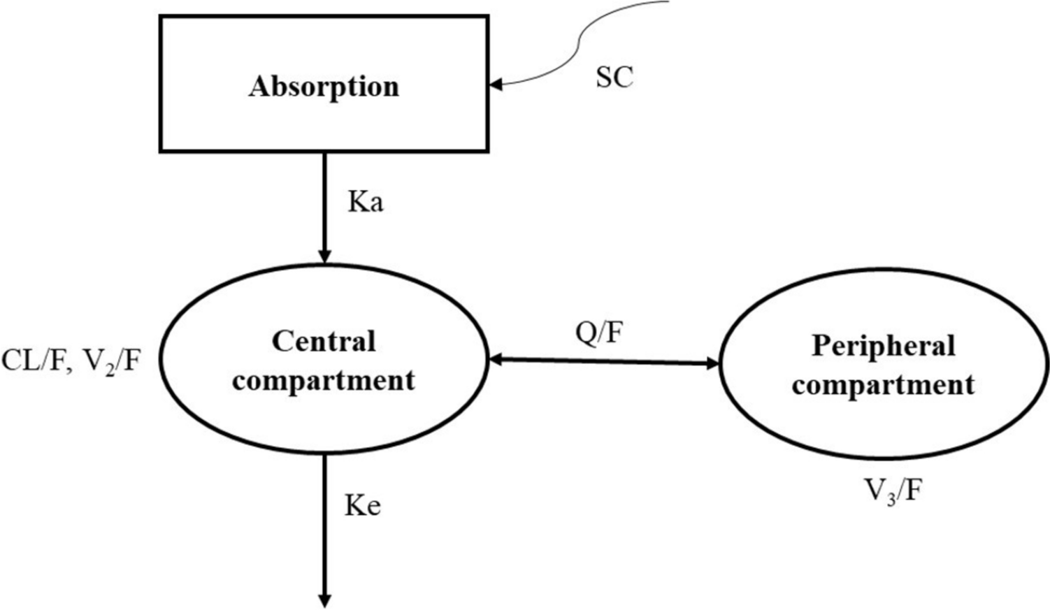
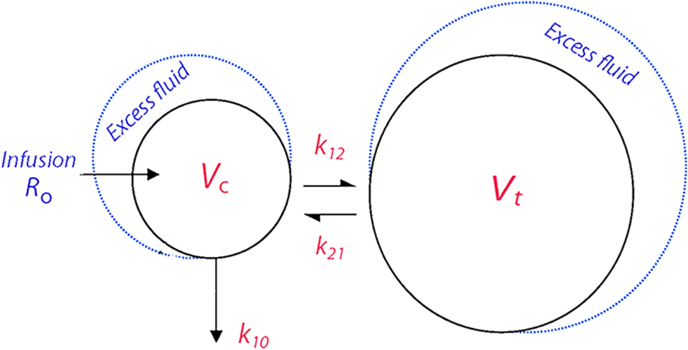
2.2 Base popPK Model

A nonlinear mixed-effects modeling approach was used for the popPK model. A two-compartment model with linear elimination and first-order absorption with lag time (Tlag) was developed. FOCE INTER was the primary method used for the estimation of model parameters.

Throughout model development, model diagnostic plots were used to assess the ability of the model to describe observed data. The plots included observed (DV) versus individual (IPRED) and population (PRED) predictions, as well as conditional/individual weighted residuals (CWRES/IWRES) and their absolute values versus PRED/IPRED. Diagnostic plot utility was dependent on a reasonable level of the inter-individual random effects and residual error. If shrinkage estimates were > 30%, plots based on random effects or residuals were interpreted cautiously.

2.2.1 Random Effects in the PopPK Model

The inter-individual random effects on the model parameters were introduced and retained when they did not cause model instability and when their estimates were not close to zero. They were modeled assuming a log-normal distribution described as follows:

$$\theta_ = \theta_ \times e^ }}$$

where θki denoted the parameter value for the ith subject, θk denoted the typical parameter value, and ηki denoted the inter-individual random effect for the ith subject, assumed to have a mean of 0 and a variance \(\omega_^.\)

The vector of random effects (across the parameters indexed by k) had the covariance matrix Ω. Covariance matrix structures, including diagonal and blocked diagonal structures, were evaluated after the completion of covariate model building.

The residual error structure was assumed to follow an additive, proportional, or combined additive and proportional error model described as follows:

$$Y_ = C_ \times \left( } \right) + \varepsilon 2_$$

where Yij is the jth observed concentration for the ith subject, Cij is the corresponding predicted concentration, and \(\varepsilon _\) (proportional) and \(\varepsilon _\) (additive) are the residual errors under the assumption that ε~N (0, σ2). The residual error model was optimized until no trends were visible in the residual plots (in particular, absolute values of IWRES vs IPRED).

2.2.2 Covariates

Baseline covariates tested were focused mainly on clinically relevant covariates and included body weight, sex, race, tumor type, age, and albumin on apparent clearance (CL/F) and apparent central volume of distribution (Vc/F); creatinine clearance, National Cancer Institute liver dysfunction category, and Eastern Cooperative Oncology Group (ECOG) performance status on CL/F; sex and tumor type on relative bioavailability (Frel); and sex on first-order absorption rate constant (Ka). Tumor type was classified as no tumor, i.e., healthy participants (reference population), mBC, or mCRC. The CYP2C8-modifying drugs were prohibited in tucatinib studies and therefore not tested in the model. Creatinine clearance was calculated according to the Cockcroft–Gault equation [13]. Covariates included in the final model were required to be available in ≥ 80% of the participants, with a minimum of 15 in each categorical covariate category. Only one of any covariates with a correlation of > 0.5 was included in the formal analysis based on the level of clinical significance or influence.

Modest increases in serum creatinine have been reported in tucatinib clinical trials including the HER2CLIMB study (HER2+ mBC). The increases were reversible, were not clinically significant, and did not result in kidney damage or treatment discontinuation. In a phase I study (SGNTUC-020), tucatinib was shown to inhibit tubular secretion of creatinine through inhibition of the organic cation transporter 2 (OCT2) and multidrug and toxin extrusion (MATE) protein renal transporters, which may cause mild increases in serum creatinine that do not result from renal impairment [11]. Thus, only baseline creatinine was included as a covariate to assess the impact of renal impairment on tucatinib PK.

Given that the effect of food on tucatinib PK was not clinically meaningful, along with the limited number of fed participants available (ARRAY-380-103, n = 11), only fasted tablet data were included and food effect was not assessed in the current popPK model [14]. ARRAY-380-103 assessed the effect of food on tucatinib PK data from 11 participants either fasted or fed a standard high-fat meal 30 min prior to administration of 300 mg of tucatinib in a crossover design. A prandial state was found to only modestly influence tucatinib exposure. The mean area under the plasma concentration–time curve from time 0 extrapolated to infinity (AUC0-inf) after a high-fat meal was increased by 1.5-fold and the Tmax shifted from 1.5 to 4 h, while Cmax was not changed [14]; this was determined to be not clinically meaningful, and tucatinib may be administered without regard to food. In the remaining studies included in the current model, all participants received their doses either in the fasted state (studies in healthy participants) or in an unknown prandial state (studies in patients with cancer where they were instructed to take their doses with or without food). Therefore, the data for tucatinib administered in the fed state in Study ARRAY-380-103 were not sufficient to assess the food effect using the popPK analysis.

A univariable screening process was used to select parameter-covariate relationships that were to be tested in the stepwise covariate search. Each parameter-covariate relationship was added one at a time to the structural model, and only parameter-covariate relationships significant at the 0.05 level in this univariable screening step or that were deemed to be of clinical significance were taken forward into the full stepwise covariate search process.

In the stepwise covariate search, covariate-parameter relationships were assessed based on forward addition with a significance level of 0.01 and backward elimination with a significance level of 0.001. During the forward addition steps, covariate-parameter relationships were added one at a time if addition led to a statistically significant model improvement, starting with the most significant relationship first. Covariate-parameter relationships were removed one at a time during the backward elimination step if deletion led to insignificant model deterioration, starting with the most insignificant relationship first.

The mathematical structures of the covariate models are shown below:

where Pki is the population estimate of the parameter Pk for subject i, Xij is the value of continuous covariate Xj for subject i (or an indicator variable for subject i for categorical covariate Xj with values of 1 for the non-reference category and 0 for the reference category), M(Xj) is the median of covariate Xj in the analysis dataset, θk is the typical value of the parameter Pk, and θj is a coefficient that reflects the effect of covariate Xj on the parameter.

2.2.3 Final PopPK Model

After covariate testing, alternative variance-covariance structures for Ω, including partial and full block structures, were evaluated. Suitable structures would provide a statistically significant (p < 0.001) improvement in the model objective function and improved model stability as measured by the condition number and/or a successful covariance step to arrive at the final model. The final popPK model criteria included successful minimization; no estimates close to the boundary; relative standard error of the estimates < 30% for fixed-effect parameters and < 50% for random-effect parameters.

2.2.4 Evaluation of the Final Model

A nonparametric bootstrap analysis, performed with 1000 replicates of the dataset generated by random sampling, was used to evaluate the stability of the final model and estimate confidence intervals (CIs) for model parameters [15]. Visual predictive checks were used for internal qualification and to evaluate the predictability of the final model [16]. Visual predictive checks were performed with prediction correction [17]. A total of 500 trial replicates were simulated using each participant’s observed covariates and dose regimens with simulated individual-specific, inter-individual, and residual variability.

2.2.5 PK Simulations

Simulations were performed using the final popPK model to predict typical PK parameters and covariate effects on tucatinib steady-state PK. Tucatinib disposition was found to be linear; therefore, the steady-state area under the plasma concentration–time curve (AUCss) was calculated using the following:

$$}_}}} = }/\left( }/}} \right)$$

where Dose is tucatinib dose and CL/F is apparent clearance of tucatinib, incorporating any covariate effects on Frel. Steady-state tucatinib Cmax and trough concentration (Ctrough) were obtained from simulated steady-state concentration–time profiles using each individual’s post-hoc parameter estimates from the final model.

Simulations of concentration–time profiles over sufficient days of BID dosing to reach steady state were performed using typical model-estimated PK parameters without including between-subject variability or residual unexplained variability to assess time to steady-state and accumulation ratios. When the AUC over the last dosing interval was ≥ 98% of the theoretical AUCss, steady-state was assumed. Area under the plasma concentration–time curve accumulation ratio was calculated as the ratio of AUC from time 0–12 h (AUC0-12) at steady-state to AUC0-12 after the first dose. The Cmax and Ctrough accumulation ratios were calculated as the ratio of the simulated maximum and trough steady-state concentration to the corresponding values after first dose. Time to steady-state was the first day that Ctrough was ≥ 95% of the simulated steady-state Ctrough.

2.2.6 Software

NONMEM® versions 7.3.0 and 7.4.3 (ICON, Hanover, MD, USA) were used for popPK modeling, and the first-order conditional estimation with interaction algorithm was used for parameter estimation. R version 4.0.4 was used for simulations. SAS version 9.4 was used for data preparation. R versions 3.6.3 and 4.0.4 were used for graphical analysis, model diagnostics, and statistical summaries. Xpose® and Pearl speaks NONMEM (PsN®) version 4.8.1 (Department of Pharmacy, Uppsala University, Uppsala, Sweden) were used for model diagnostics and facilitation of tasks such as covariate testing and bootstrap.