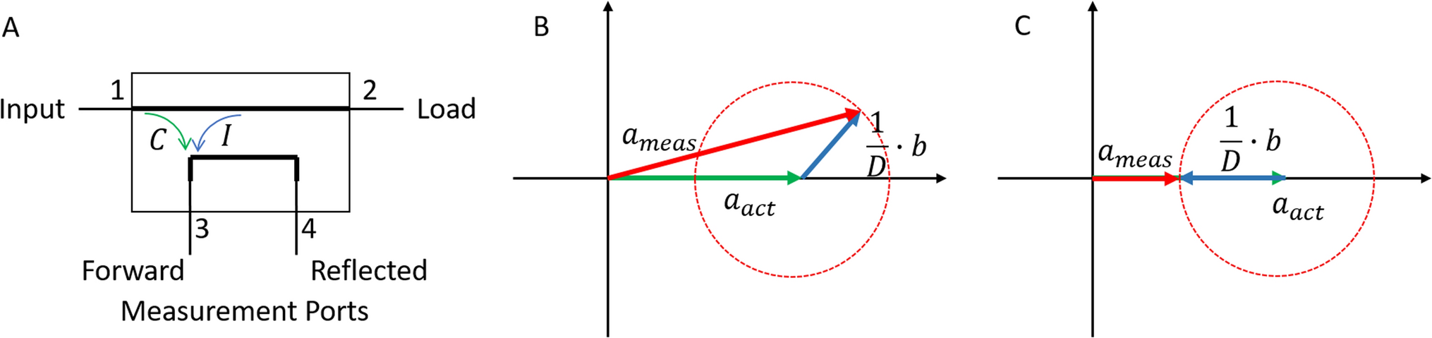
A simplified example of a directional coupler [9] is shown in Fig. 1A. The signal is transmitted from Port 1 (Input) to Port 2 (Load, e.g., antenna). A portion of the signal entering Port 1 is coupled to Port 3 with a coupling coefficient \(C\) and a smaller part from Port 2 to Port 3 with an isolation coefficient \(I\). The ratio between these two coefficients is called directivity \(D\). An ideal directional coupler would have an isolation coefficient \(I\) of 0 and therefore an infinite directivity.

A Simplified schematic of a directional coupler. B Vector representation of measured signals at a coupled port of a directional coupler. C Worst-case phase, where the measured signal \(_}\) is minimal because \(_}\) and \(b\) have opposed phase

Due to the finite directivity of real-world directional couplers, the measured complex forward voltage signal \(_}\) consists of the summation of the signal we would ideally measure \(_\) and the reflected signal \(b\) weighted with the inverse of the directivity \(D\):

$$_}=_}+\frac\bullet b$$

(1)

Since \(_}\) and \(b\) are vector representations of complex signals, the measured signal also depends on the phase between \(b\) and \(_}\). Therefore, the result for \(_}\) for a certain amplitude of \(b\) is somewhere on the dashed circle in Fig. 1B.

The worst-case error, meaning the largest underestimation of SAR, for a measurement with a directional coupler and a single transmitter is shown in Fig. 1C, where \(_}\) and \(b\) are 180° out of phase. In this case, the measured forward signal is smaller than the actual forward signal, leading to an underestimation of SAR. Since the maximum possible reflected power in a single-channel system is identical to the applied forward power and the directivity is known, the worst-case underestimation can be calculated directly and compensated for.

For parallel transmit systems, the calculation of a worst case is much more difficult. First, the SAR not only depends on the amplitude of the forward signal, but also on its phase and is therefore a function of the complex excitation vector \(}\), whose number of elements is equal to the number of channels. Here, each complex entry in the excitation vector corresponds to a complex signal \(_\) as introduced above. Second, the total reflected power in a channel is a function not only of the forward power in this channel, as in a single-channel system, but also depends on the amplitudes and phases of the signals from the other channels coupling into this channel. The latter contributions can be significantly higher than the channel’s own internal reflection [10].

In practice, the excitation vector \(\mathbf\) containing the complex signals for all channels is measured using directional couplers between the amplifiers and the RF array. Due to the finite directivity \(D\) of the directional couplers, the measurement yields the values

$$}}_}=\frac\bullet }+}}_}$$

(2)

where \(\mathbf\) is the complex vector of the reflected signals. Each complex entry of \(}}_}\) now corresponds to the respective \(_}\) of the channels.

With the complex S-parameter matrix \(\mathbf\) of an RF array [11] and the complex excitation vector \(}}_}\) of a multi-channel system, the vector of the complex reflected signal \(\mathbf\) can be calculated as

$$}=\frac^\mathbf}}_}$$

(3)

Here, the term \(^\) describes the potential phase difference between the planes of reference of the S-parameters (for example from a simulation) and the directional coupler measurement. We use a single phase for all channels, as it is a reasonable assumption that cable length is close to identical. Furthermore, \(\frac\) describes the extra attenuation introduced by the cable between the points of S-parameter measurement and directional coupler measurement. With these two terms, we can effectively shift the measurement of the forward power along the transmit cable. This is necessary as our results show that the exact position of measuring the forward power is important for the error.

With Eq. 3, the measured excitation vector can be written as

$$}}_}=e}^\frac\bullet \mathbf}}_}+}}_}$$

(4)

Generally, the directional couplers are placed as close to the coils as possible. As the attenuation over a length of less than one wavelength is fairly low in the transmit cables of an MRI system and therefore negligible compared to the directivity and is in any case equivalent to a slight increase in directivity, we disregard it in the further steps.

As stated in the introduction, to calculate the local SAR in the online supervision of a multi-channel MRI system, often so-called virtual observation points (VOPs) are used [7] that are derived from Q-matrices [12]. With the VOP matrices \(}_}}\) of the VOP set \(}_}\) and the complex excitation vector \(}\), SAR in the volume of the virtual observation point \(j\) can be easily calculated as

Since the measured excitation vector is different from the actual excitation vector, the SAR calculations yield different results

$$}_}=}}_}^}_}}_}=^\frac\bullet \mathbf}}_}+}}_}\right)}^\mathbf}_\left(^\frac\bullet \mathbf}}_}+}}_}\right)$$

(6)

In this form, it is not easy to compare the SAR calculated from the measurements to the actual SAR.

Using a few simple steps, Eq. 6 can be reformulated as follows:

$$\begin }_}}} = & \left( \frac \cdot }}_}}} + }_}}} } \right)^ }_ \left( \frac \cdot }}_}}} + }_}}} } \right) \\ = & }_}}}^ \left( \frac \cdot } + }} \right)^ }_ \left( \frac \cdot } + }} \right)}_}}} \\ \user2 = & }_}}}^ }_}}}^ }_ }_}}} }_}}} \\ = & }_}}}^ }}_}}} }_}}} \\ \end$$

(7)

Here, \(\mathbf\) is the identity matrix and we designate \(}_}\) the error matrix. Through the above reformulation, we now have a new set \(}_\) of VOP matrices \(}}_}\).

In the following, we use \(k\) instead of j as the running index to avoid confusion with the running index \(j\) of the original set of matrices \(}_}\); nevertheless, a matrix \(}}_}\) is derived from \(}_\) if \(k=j\). We can easily compare \(}}_}\) of \(}_}\) to the actual SAR matrices \(}_\) of \(}_}\) for all possible values of \(}\in }^_}\) using the CO criterion introduced by Gras et al. [8]: to find the maximum relative error \(r\) introduced by the measurement with directional couplers, we now need to solve

$$r\left(\phi \right)=\underset}_\in }_}}}\underset}\in }^_}}}\left(}}_}\in }_}}}\left(}}^\left(}}_}\right)}\right)\right)}^}}^}_}\right)$$

(8)

The maximization over \(\mathbf\) can be reformulated as

$$r_}}} \left( }_ ,\phi } \right) = \mathop \limits_} \in }^ }} }} \left( }^ }_}}} }} \right)\;}\;}\;}^ }}_},}}} } \le 1,\user2\forall }}_}}} \in }_}}}$$

(9)

with

$$}_}}} = \left( c} }\left( }_ } \right)} & \left( }_ } \right)} \\ \left( }_ } \right)} & }\left( }_ } \right)} \\ \end } \right)\;}\;}}_},}}} = \left( c} }\left( }}_}}} } \right)} & \left( }}_}}} } \right)} \\ \left( }}_}}} } \right)} & }\left( }}_}}} } \right)} \\ \end } \right)$$

(10)

Gras et al. showed in their paper that this is a convex problem [8]. The maximum over \(}_\in }_}\) can be calculated by running the inner optimization for each element of \(}_}\) and choosing the maximum.

Since finding the maximum error over the phase difference between the reference planes of the S-parameter measurements and the directional coupler measurements is not a convex problem as our results will show, we run the phase difference \(\phi\) from 0 to 2π in 360 steps.

To provide an impression on how large the error can be for different arrays and how much it varies, we used simulation data of five different RF arrays with realistic human body models from CST Microwave Studio (Dassault Systèmes, Vélizy-Villacoublay, France). Four of these are 7 T arrays: a fractionated dipole [13] head array with eight channels (FD 8ch), a rectangular loop head array with eight channels (RL 8ch), a 32-channel integrated body array of microstrip lines with meanders [14] (MSM 32ch), and an 8-channel flexible body array of microstrip lines with meanders [15] (MSM 8ch). Furthermore, a microstrip line body array for 3 T (3T MS 8ch) very similar to the work of Vernickel et al. [16] was simulated. Images of the CAD models are shown in Fig. 2. The SAR matrices were exported to Matlab and compressed using hybrid compression algorithms [17]. S-parameters were exported to calculate the error matrices. Since it is clear from Eq. 5 that the S-parameter matrix plays an important role for the extent of the error in the measurement, the eigenvalues of \(}^\mathbf\) were calculated according to the work of Kazemivalipour et al. [10]. This provides information on the total reflected power, with the highest eigenvalue providing the worst-case total reflected power. The eigenvalues can be used as a quality measure for the coupling of an array.

Coil array models used in this work. FD 8ch is a large head array consisting of 8 fractionated dipoles, RL 8ch is a large head array consisting of rectangular loops, both for 7 Tesla. 3T MS 8ch is an 8-channel body array for 3 Tesla consisting of 8 microstrip lines. MSM 32 is an integrated body array for 7 Tesla consisting of 32 microstrip lines with meanders, while MSM 8ch is local body array consisting of the same element type

Two types of errors were investigated: 1) the maximum underestimation of local SAR was calculated as explained above, and 2) the maximum underestimation in the measurement of total forward power was evaluated by calculating one over the minimum eigenvalue of \(}_}=\mathbf}_}}^}_}\). The second calculation is identical to using an identity matrix instead of a set of VOPs for the calculation of \(r\).

All calculations were performed in Matlab R2023a (The MathWorks, Natick, MA, USA).