2.1 Hardware

All measurements were conducted using a clinical 3 T MR system (MAGNETOM Prisma-Fit, Siemens Healthineers, Erlangen, Germany) equipped with external multi-channel body and spine phased-array coils for signal reception.

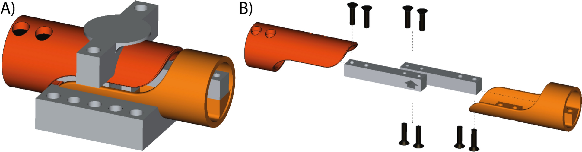
The experimental setup featured a custom-designed 16-channel external add-on shim coil array, structured into four distinct "shim" modules (Dia, MR Shim GmbH, Reutlingen, Germany). The geometry, shape, and number of turns of the shim coils were selected to achieve maximum coverage while taking into consideration the available space and mechanical constraints of the MRI setup. The shim coils have a standard circular shape, and the number of turns and size (20 turns and 6 cm diameter) were chosen such that the shim coils can fit inside the shim holder while keeping the thickness of the shim holder below 1 cm, and to ensure that the required current for each channel remains below 1 A. The shim cables were made with 20 AWG wires as twisted pairs.

The shim coil setup included eight channels on the anterior side, divided into two modules (blue frames in Fig. 1a), and eight channels on the posterior side, distributed across two modules (red frame in Fig. 1a), for full coverage. On the posterior side, the eight channels were uniformly distributed within the available space of the patient bed using a shim coil holder with a width of approximately 35 cm. The main patient mattress normally sits on top of the spine coil housing, so the positioning was achieved by placing the channels below the mattress but above the spine coil. To maximize coverage, the eight shim coils were arranged in two rows, resulting in a shim coil holder length of ~ 16 cm. For the anterior coils, the shim holder design was constrained by the shape of the body array receive coil, to which the coils were mechanically fixed. A configuration of two columns was chosen (four shim coils in each column in a shim holder covering a span of approximately 38 cm in the head-foot direction). To configure this setup, the anterior modules were positioned on the 18-channel RF body receive array coil, while the posterior modules were positioned underneath the patient's bed mattress on top of the RF spine-array coil, as indicated in Fig. 1b. Each rigid shim module had fiducial markers embedded in the housing, enabling the detection of the position of the shim coils for each subject.

Fig. 1

Experimental setup of an external shim coil array. a the 16-channel local shim coil array, consisting of two posterior modules (red frame) and two anterior modules (blue frame). The anterior modules are positioned on top of the external RF 18-channel body phased-array coil. b System configuration. The anterior shimming modules (blue) are positioned around the receive RF coil and the posterior modules (red) are placed under the mattress of the patient bed. The shim modules are connected to the filtered shim interface box. c the maximum field strengths of the coil elements observed in vivo within the prostate of a representative volunteer at a current of 1 A

A filtered shim interface box was positioned at the head of the scanner table. This interface box served as the central hub for the connection of the four shim modules. To drive the shim coils with electric currents, two amplifier units (Jupiter, MR Shim GmbH Reutlingen, Germany) were deployed. These amplifier units were positioned in the corner of the scanner room situated beyond the 100 Gauss line. Adjacent to the amplifier units, a non-magnetic Ethernet-to-fiber optic converter box was powered by a 5 V power adapter, which was also connected to the mains supply. The box was linked to the master shim amplifier unit through a short Ethernet cable, and to its counterpart outside of the magnet room positioned next to the host computer using a duplex fiber optic cable. This cable was threaded through the waveguide opening of the MRI room penetration panel, ensuring an interference-free connection. In the MRI control room, the Fiber optic-to-Ethernet converter box was powered using a 5 V power adapter and connected to the shim controller PC through an Ethernet cable.

Figure 2 illustrates the field patterns generated by each local shim coil across the prostate and B0 map distributions generated by each coil are shown in Supplementary Fig. 1. Depending on the position of each local shim coil relative to the prostate, the coils were able to produce a peak-to-peak variation of between 36 to 129 Hz over the extent of the prostate region. The maximum field strength produced by each of the local shim coils across the prostate for 1A of shim current is also summarized in the table of Fig. 1c.

Fig. 2

Strength and penetration depth of the local shim array. The line profile of the magnetic field created by each of the 16 local shim coils at 1A of shim current on a representative volunteer are plotted (red) for the head-foot (HF), anterior–posterior (AP) and right-left (RL) directions. As a comparison, the line profile of the magnetic fields created by scanner’s 2nd order spherical harmonic shim values set at 1000 μT/m2 is also shown (blue). The curves for the local shim coils illustrate changes in the order of microTesla over distances of 30 to 50 mm. Changes of 1 microTesla can result in a frequency difference of up to 40 Hz, and when multiple elements are combined, they can counteract inhomogeneities on the order of 150 Hz

Acquisition protocolSubjects

We examined seven healthy volunteers (V1 to V7), with a mean age of 40.7 years (range 28 to 65 years). These volunteers underwent scanning without any prior bowel preparation. Ethical approval for the study was obtained from the local ethical committees at Radboudumc, Nijmegen, the Netherlands.

Shimming procedures

All of the supplementary hardware described above was operated via a controller PC utilizing the Arche shimming software (MR Shim GmbH Reutlingen, Germany).

The shimming procedures using the 16-channel add-on local shim coil in combination with the scanner’s shimming system involved the steps outlined below and depicted in Fig. 3, to achieve a high 3D volumetric magnetic field homogeneity around the prostate.

Fig. 3

Flowchart providing an overview of the shimming process. Left: the add-on shim coil procedure Right: conventional shimming procedure

For experimental shimming with the shim coil array, we identified a rectangular in vivo volume, indicated for B0 homogeneity optimization, known as the adjustment volume. This volume was precisely positioned on T2W localizer images, on the scanner’s host PC and software, selecting the prostate while minimizing the inclusion of surrounding tissues. Next, a double echo gradient echo pulse sequence was acquired for offline mapping of the B0 field within the adjustment volume. After obtaining the B0 field map, the optimal combination of 1st-order shim values of the MR scanner along with the settings for the add-on shim coil array was calculated on the shim controller PC. The higher-order shim values of the MR scanner were left unchanged at the tune-up values. To minimize B0 field disturbances within the adjustment volume, we used a least-squares minimization approach of the sum of the original B0 field heterogeneity and the targeted combined B0 shim field of the 1st-order scanner shims and the add-on shim coil array. The shim values were computed using a non-iterative approach via the Arche shim software, which employed a constrained convex optimization algorithm. Once calculated, these shim values were applied to the scanner’s 1st order shims in the interactive Adjustments window, and to the corresponding shim array amplifiers and coils on the separate shim controller PC.

As a reference standard, we used the MR scanner's 3D map shimming routine to calculate all available shim values (1st and 2nd order), specifically optimized for the prostate, following the protocol used in clinical routine. This was complemented by manual fine-tuning, where an experienced spectroscopist made interactive adjustments to the scanner settings. Our consistent goal during manual fine-tuning was to achieve a magnitude full width at half maximum (FWHM) of approximately 30 Hz within the adjustment volume around the prostate. In many instances, we achieved better results, well below the 30 Hz target.

The MR scanner's 3D map shimming routine settings were adjusted using the scanner’s clinical “fine-tune” routine, which minimizes the FWHM of the water resonance in the prostate. In contrast, add-on local shim coil array optimization minimized the ΔB₀ standard deviation within the prostate VOI. While the two methods use different metrics, this reflects the available control for each system.

Imaging protocol

The anterior modules of the add-on shim coil were fixed to the RF body receive array coil, while the posterior modules were fixed under the mattress of the patient bed. During subject positioning, care was taken to ensure the optimal placement of the prostate between the anterior and posterior shim coils.

The MR acquisition protocol and associated settings are detailed in Table 1. The acquisition procedure consisted of localizer scans, B0 field maps, T2-weighted (T2W) imaging, DWI, and 1H-MRSI. B0 field maps were acquired with a dual-echo gradient echo sequence. The anatomical T2W scans were obtained in three orthogonal orientations using a clinical turbo spin-echo (TSE) pulse sequence. For DWI, we employed a spin-echo EPI sequence with a b-value of 50 s/mm2 and repeated the sequence with b-values 50, 400, and 800 s/mm2, from which an image corresponding to a b-value of 1400 s/mm2 was calculated.

Table 1 The MR acquisition protocol and associated settings

The 3D 1H-MRSI acquisition, a semi-LASER sequence with gradient offset independent adiabaticity (GOIA) pulses was used [34]. A slice-selective Shinnar-Le Roux optimized 90° excitation pulse (duration 4 ms) was followed by two pairs of refocusing pulses. The GOIA refocusing pulses with WURST(n,m) modulation had a duration of 8 ms, a bandwidth of 3 kHz, a maximum B₁ amplitude of approximately 718 Hz, and a gradient modulation factor of f = 0.9. The echo time (TE) was set to 88 ms. Lipid and water signal suppression was achieved using MEGA editing pulses placed after the first GOIA refocusing pulse. The MEGA pulses had a bandwidth of 1.6 ppm, a duration of 12.8 ms, and an RF amplitude of 260 Hz. Outer volume suppression bands were placed around the prostate volume to minimize lipid contamination. The acquisition matrix was an elliptically sampled k-space matrix of 8 × 8 × 11 phase encode steps zero filled to 16 × 16 × 16 after hamming filtering.

To minimize effects of motion between separate parts of the examination and to compare the two shimming approaches (add-on coil array vs reference standard), the shimming procedure was repeated twice during the protocol, involving separate B0 field acquisitions and recalculating shim values before both the DWI acquisition and the 1H-MRSI pulse sequence in both separate shimming approaches.

Shim coils calibration

Reference B0 field maps from each individual shim coil were acquired on a phantom and served as the reference calibration data set. The positions of the shim modules with respect to the system’s isocenter and the subject’s prostate during each pursuing scan session were detectable on T2W localizer images by the fiducial markers embedded in the housing. As these shim modules vary in each subject and table position from the initial phantom shim coil calibration session, detection of fiducial markers on T2W localizer images for each subject is crucial. This was done manually by the user in the shim software (MR Shim, Germany) graphical user interface (GUI). Using these newly identified fiducial marker locations, rigid transformations, encompassing translation and rotation, were automatically calculated utilizing singular-value decomposition[35], and the magnetic field generated by each shim coil was calibrated to match the current position and orientation of the markers in each subject[36]. The total overhead calculation time when using the add-on shim system (including data transfer, fiducial marker detection and shim calculation) was approximately 2 min.

Initial proof of concept

In this study a total of 16 local shim coils and the scanner-provided 1st and 2nd order spherical harmonic shim coils were available. Theoretically, the higher the number of employed shim coils, the more uniform the achievable shimmed field. In the initial stages of this work, we indeed used all available shim coils (add-on + 1st + 2nd order spherical harmonics) for shimming, illustrating a successful proof-of-concept implementation of the add-on shim array (Supplementary Fig. 2, vol A). However, very variable results were acquired, with cases in which the measured shimmed magnetic field map deviated substantially from the predicted maps (Supplementary Fig. 2, vol B: the measured field map after shimming deviated from the predicted value by more than 7 Hz).

Suspecting a disadvantageous interaction between possibly imperfect higher-order spherical harmonic fields, bowel motion and our add-on shim array we hypothesized that the 2nd order shims, while theoretically improving field homogeneity in the VOI, may reduce robustness against bowel motion. The magnetic fields generated by higher-order spherical harmonic coils are known to rapidly drop off further from the iso-center due to their geometry. This rapid drop-off contributes to a very inhomogeneous field outside the volume of interest (VOI) when shimming smaller regions of interest. This not only increases the chance of failure of global lipid/water suppression pulses and/or contributes to spurious signal stemming from outside the VOI in spectroscopy studies [37], but will additionally make the shim quality very susceptible to perturbations caused by motion.

Therefore, we simulated the robustness of two different shim strategies against motion, as described in Sect. "Initial proof of concept" and concluded that using the add-on shim coils in combination with only 1st order spherical harmonics shims of the scanner was the preferred way to go.

Shim strategy for robust and motion-insensitive shimming

A simulation study was conducted to assess the robustness of two different shim strategies:1) using the add-on shim coils in combination with only 1st order spherical harmonics (add-on + 1st), 2) using the add-on shim coils in combination with both 1st and 2nd order spherical harmonics (add-on + 2nd).

Reference B0 maps from 5 healthy volunteers were used for the simulation study. First, the theoretically best attainable shim quality in the prostate region for each shim configuration was calculated. The resulting field homogeneity (as measured by the standard deviation of the frequency offsets) was compared between the two shim configurations both inside the prostate and in the immediate ± 2 cm outside the prostate in each direction. Figure 4 illustrates the bar plots of the calculated values for each setting. The shim optimization aimed to minimize the standard deviation of ΔB₀ within the prostate VOI using a least-squares approach.

Fig. 4

Comparison of simulated shim quality. For each volunteer, the standard deviation of the frequency offsets in the simulated shimmed map (both inside the prostate region and in an immediate ± 2 cm volume outside the prostate) are shown for two different shim configurations

Τhe second shim configuration (add-on + 2nd order spherical harmonics) results in a better shim quality inside the prostate region (on average 1.67 Hz better than the add-on + 1st shim configuration across all volunteers). However, invariably, this advantage inside the VOI comes at the price of a worse field homogeneity in the immediate region outside the prostate (on average 13.5 Hz worse than the add-on + 1st shim configuration across all volunteers). As an example, the resulting shimmed field maps inside and outside the prostate region are shown in Fig. 5 for two representative volunteers.

Fig. 5

Plots of simulated shimmed maps inside and outside the volume of interest of the prostate. Simulated shimmed B0 maps overlaid on anatomical reference images are shown for two representative volunteers. The addition of 2nd order shims from the scanner introduced larger field deviations immediately outside the VOI (outside green box, within yellow box). The shimmed maps are shown for two different shimming configurations (add-on + 1st vs. add-on + 2nd). For each case, the maps of both inside (green box) and outside (yellow box) of the prostate region are shown. Green arrows point to areas where the inclusion of 2nd-order shims have resulted in an improvement inside the VOI. Red arrows point to areas with extreme and rapid field drop-off of field homogeneity outside the VOI

Next, the robustness of each shim configuration against motion was assessed. A range of ± 1 to ± 9 mm displacement in each three directions (anterior–posterior, right-left, and head-foot) was considered. For each displacement, it was assumed that the underlying magnetic field is displaced by motion, but the prescribed imaging volume stays the same, as no prospective motion correction is employed. The effect of the motion on the shim quality of the original prostate position was calculated and compared for the two shim configurations. Additionally, another scenario where the anterior local shim coils (the only movable part of the shim system) also moves with the patient was considered for each case.

Figure 6 shows the bar plots of the aggregated results showcasing how much the resulting field homogeneity deviates from the “reference” shim in each case. The reference shim is the best achievable shim using all available shim coils in a no-motion scenario (i.e. add-on + 2nd). It is important to study this metric since the goal here is to challenge the assumption that the configuration resulting in the reference shim in a no-motion scenario should be used without question. The goal is to understand how quickly each shim configuration strays from this reference as a result of even small amounts of motion. The results confirm that in every case the add-on + 1st shim configuration stays much closer to the reference shim. However, the add-on + 2nd order shim quickly loses its original advantage and results in a much worse shim, with an average deviation of 3.2 Hz across all volunteers and motion cases (compared to 1.1 Hz for the add-on + 1st scenario).

Fig. 6

Susceptibility of shim quality to perturbations caused by motion. For each volunteer, the bar plots show the resulting aggregated shim quality for each shim configuration simulated over a range of motion (± 1 mm to ± 9 mm) in each three directions (AP,RL,HF). An additional scenario where the anterior shim coils also move are also shown. Each bar represents the deviation of the shim quality from the reference shim

In light of this simulation study, the add-on + 1st shim configuration was chosen as the method of choice for the test of this study, as it resulted in a more stable shim and a more homogeneous field in the immediate region outside the VOI.

Influence of add-on shim coil array on MR system performance

Tests were conducted using the homogeneous Siemens spherical D240 body loader tissue phantom to ensure compliance with performance criteria outlined by the National Electrical Manufacturers Association (NEMA) and the Acceptance Testing and Quality Assurance Procedures for Magnetic Resonance Imaging Facilities (AAPM). These tests aimed to evaluate RF interactions resulting from the presence of the shim coils. Measurements were conducted using body and spine array coils for signal reception and were performed twice: once with the shim coils present but without current running through them, and once without the shim coils.

Flip angle maps were obtained using the turbo flash B1 + mapping product sequence (tfl_b1map) with the following parameters: TR/TE 5280/1.8 ms, field of view (FOV) 300 × 300 mm2, base resolution 64 × 64.

Additionally, a 2D multi-slice T2-weighted (T2W) spin echo pulse sequence was employed with the following parameters: TR/TE 6000/96 ms, field of view (FOV) 350 × 350 mm2, 70 slices of 3.5 mm, and base resolution 256 × 256. From these images, the following parameters were assessed:

1. the signal to noise ratio (SNR), were a noise region and signal (S) region (Supplementary Fig. 3) where selected on the slice on iso-center and SNR was calculated according to

where σ is the standard deviation of the noise in the noise region.

2. percentage of signal ghosting, where a signal region (S), and two sets of background regions (one in the frequency-encoding direction (SFE1, SFE2) and one in phase-encoding direction (SPE1, SPE2)) (Supplementary Fig. 4) were selected on the slice at iso-center and the percentage ghosting signal was calculated, through the ghosting ratio (GR), according to.

$$GR=100\left|\frac_}+ \overline_} \right)- \left(\overline_}+\overline_} \right)} }\right|$$

(2)

Analysis

The analysis of the B0 and DWI data was conducted using Matlab (version 9.11 R2021b; MathWorks, Natick, MA).

B0-maps

To quantitatively assess B0 homogeneity, the standard deviation (SD) of off-resonance frequencies (ΔB0) was calculated per slice of the B0 maps within the Adjustment Volume.

The local ΔΒ0 variation was computed from the phase difference of the two acquisitions within a double gradient echo sequence with the parameters given in Table 1 [1]. The SD of the ΔΒ0 values was computed over the rectangular adjustment volume used for the second-order shimming, both on a slice-by-slice basis for each volunteer and over the entire volunteer cohort.

DWI analysis

The two image series with b-value of 50 s/mm2 (b50-maps) acquired with the add-on shim coil and with conventional shimming were by rigid registration matched to the transversal T2W scan as an undistorted anatomical reference, with interpolation of the EPI images to ensure resolution matching. A single reader manually segmented the entire prostate gland on each slice across the T2W series and the two b50-maps of both shimming methods. The contours of the b50-maps were aligned to the T2W images by matching the centroids of the corresponding contours.

Subsequently, the Dice similarity coefficient (DSC) [38, 39] was calculated to assess the agreement of the outlined prostate between both b50-images with the anatomical T2W images. In the DSC metric, the closer a value is to 1, the more precise the geometry of the prostate aligns in the b-50 DWI images as well as in the T2W images. This analysis was conducted on a slice-by-slice basis for each volunteer and for the entire cohort of volunteers. Statistical significance of the DSC’s was determined by a paired analysis using the Wilcoxon signed-rank test.

1H-MRSI analysis

Spectroscopic imaging data were analyzed by quantifying the citrate (Cit) peak, a metabolite abundant in the prostate, and measuring its linewidth as an indicator of spectral quality. Fitting was performed using AMARES within the jMRUI software [40]. Although Cit consists of a strongly coupled spin system with a pulse sequence timing and B0 field-dependent complex line shape, we could model the center two lines of this shape with two coupled Lorentzian line shape models. This way, the possible presence of individual variation in the small satellite signals around the two central lines does not interfere with the linewidth assessment. In the fitting procedure, all spectra within the volume of interest (VOI) were included, followed by a quality control (QC) step. Spectral fits with a Cramer Rao Lower Bound (CRLB) of the linewidth smaller than 20% were accepted as good estimates of the linewidth. The percentage of the spectra passing the QC in both shimming techniques was calculated. Spectra that satisfied the QC criterion in both shimming protocols were retained for subsequent analysis steps. To assess the statistical differences in Cit linewidth between the two shimming techniques, a paired t-test for statistical evaluation was performed, both on an individual volunteer basis and for the entire volunteer cohort. To assess the overall quality of the MRSI datasets, a scoring system based on the expert consensus paper [4] was created. The following guidelines on FWHM of spectroscopy in the prostate at 3 T are established in that paper:

5 < mean FWHM < 8: Excellent

8 < mean FWHM < 11: Adequate

11 < mean FWHM < 14: Acceptable

Based on this guideline a scoring system is devised, which takes into account not only the mean but the standard deviation (spread) of the FWHM values distributed across the prostate:

$$Score=100- \frac*80-\left(\sigma FWHM-1.5\right)*10$$

(3)

The scoring system has a linear penalty for deviation of the average FWHM from 6.5 Hz (mean of excellent score according to the consensus paper). Additionally, there is a term penalizing the high spread of FWHM values in the VOI (> 1.5 Hz which is the acceptable spread in each of the consensus system tiers). A wider distribution of FWHM values indicates heterogeneity in the data and reduced reliability of the overall spectroscopic information. The scoring formula reflects the expert guidelines by assigning a high score (100) for either a FWHM distribution of 8 ± 0 Hz or 6.5 ± 1.5 Hz.

The scores for each MRSI dataset were calculated and compared. Additionally, exemplary Cit linewidth metabolite maps for three slices from a single volunteer were generated, and histograms were created to visually depict the distribution of Cit linewidths among the volunteers.