Protein coabundance scores genome-wide protein associations

We started by collecting protein abundance data from proteomics studies of cohorts of participants with cancer. In total, we compiled a dataset of 50 studies across 14 human tissues, encompassing 5,726 samples of tumors and 2,085 samples of adjacent healthy tissue26,27,28,29,30,31,32,33,34,35,36,37,38,39,40,41,42,43,44,45,46,47,48,49,50,51,52,53,54,55,56,57,58,59,60,61,62,63,64,65,66,67,68,69,70,71,72,73,74,75 (Fig. 1a and Supplementary Table 1). We further included the mRNA expression data paired to the proteomics for 2,930 of the tumor and 722 of the healthy samples. Following previous studies, we used the fact that protein complex members are strongly transcriptionally and post-transcriptionally coregulated to compute probabilities of protein–protein associations from the abundance data5,17,20 (Fig. 1b, Methods and Supplementary Fig. 1). In short, we preprocessed the abundance data to obtain a log-transformed and median-normalized abundance across participants. For each study, we then computed a coabundance estimate of a protein pair as the Pearson correlation when both proteins were quantified in at least 30 samples (Supplementary Fig. 2). Lastly, with pairs of subunits for curated stable protein complexes as ground-truth positives (CORUM76), we used a logistic model for each study to convert the coabundance estimates to probabilities of protein–protein associations (Supplementary Figs. 3–5).

Fig. 1: Protein coabundance outperforms mRNA coexpression and protein cofractionation for recovering protein–protein interactions on a genome-wide scale.

a, Number of tumor and healthy samples per tissue. Bar sections indicate individual studies, using multiplexed proteomics with isobaric labeling (dark blue) or other methods (light blue). b, Schematic representation of workflow. Subunits of protein complexes occur in fixed stoichiometries. Protein coabundance is estimated through correlation of protein abundance profiles and converted to probabilities through a logistic model using interactions between subunits of protein complexes (CORUM) as positives. Degr., degradation. c, ROC curves for association probabilities in lung tissue derived from protein coabundance (coabund.; blue), mRNA coexpression (coexpr.; orange) and protein cofractionation (cofrac.; green). The gray dashed line shows the performance of a random classifier. FPR, false-positive rate; TPR, true-positive rate. d, AUC values for association probabilities as illustrated in c. Shown are studies that quantified both protein coabundance (blue; n = 29) and mRNA coexpression (orange; n = 29) or protein cofractionation (green; n = 10). e, AUC values for association probabilities derived from protein coabundance combined with mRNA coexpression through a linear model (purple) and protein coabundance after regressing gene expression out of the protein abundance (pink). Shown are the same studies as in d. In d,e, each dot represents one study with paired transcriptomics and proteomics data. Protein pairs were filtered for having association probabilities from both modalities. Error bars show the mean and s.e.m. In c–e, negatives are all quantified protein pairs not reported as complex members. f, Clustering of the n = 48 cohorts using association probabilities of protein pairs with the most variable associations (CV above the median). The radial dendrogram shows complete-linkage clustering with the Pearson correlation distance. Cohorts are labeled according to the type of cancer; colors represent the different human tissues. Leaf-joint distances were shortened. g, Heat map of AUCs for recovering tissue-specific associations with cohorts that were withheld when predicting these associations. Each square represents the average AUC for all cohorts of a given tissue. Tissues were clustered through complete-linkage clustering with the Manhattan distance.

Source data

To test the ability of the association probabilities to recover known complex members, we computed receiver operating characteristic (ROC) curves for probabilities derived from protein coabundance, mRNA coexpression and protein cofractionation6,7,77 (Fig. 1c). We found that protein coabundance (area under the curve (AUC) = 0.80 ± 0.01 (mean ± s.e.m.)) outperformed protein cofractionation (AUC = 0.69 ± 0.01) and mRNA coexpression (AUC = 0.70 ± 0.01) data for recovering known interactions (Fig. 1d and Methods). In addition, the combination of mRNA and protein abundance data did not significantly improve the recovery of known complex members (Fig. 1e; AUC = 0.82 ± 0.01, P = 0.15, according to a one-sided Welch’s t-test). Therefore, with roughly half of all cohorts having paired mRNA expression data available, we chose to only use protein coabundance for computing association probabilities. Additionally, we found similar AUCs when regressing gene expression out of the protein abundance before computing protein coabundance estimates (AUC = 0.78 ± 0.01, P = 0.18), suggesting that post-transcriptional processes but not regulation of gene expression drive most of the predictive power for protein associations.

Having established that the association probabilities derived from protein coabundance data recover known interactions of protein complex members, we sought to test whether replicate studies of the same tissue yielded association probabilities that were representative for each tissue. As a starting point, we used the gene expression data to establish that the association probabilities were not driven by cell-type composition78 (Supplementary Fig. 6). Next, using the 1,115,405 association probabilities that were quantified for all studies, we found that the replicate cohorts from the same tissue generally clustered together (Fig. 1f; for example, blood, brain, liver and lung). Next, we selected the associations that were tissue specific, that is associations whose average probability exceeded the 95th percentile for a given tissue (0.68 ± 0.01 across tissues) and whose average probability remained below 0.5 across all other tissues. Through a hold-one-out methodology, we found that the tissue-specific associations were primarily recovered by cohorts of the same tissue of origin (AUC = 0.71 ± 0.01) compared to cohorts from different tissues (AUC = 0.56 ± 0.00, P < 0.05 for all tissues, according to a one-sided Welch’s t-test) (Fig. 1g, Methods and Supplementary Fig. 7). Together, these observations suggest that the tissue of origin is a major driver of differences between cohorts.

An atlas of protein associations in human tissues

With the replicate cohorts representing the tissue of origin, we aggregated the association probabilities from cohorts of the same tissue into single association scores for 11 human tissues (Fig. 2a and Methods). Aggregating the replicate cohorts was advantageous, as all but one of the individual cohorts were outperformed by the tissue-level scores for recovering known protein interactions (P = 1.3 × 10−9, according to a one-sided Welch’s t-test). Moreover, the tumor-derived scores outperformed the healthy-tissue-derived scores for all tissues (Fig. 2b; AUC = 0.87 ± 0.01 and 0.82 ± 0.01, respectively, P = 8.3 × 10−5, according to a one-sided Welch’s t-test). In addition to the biopsy, where the genetic heterogeneity of tumors increased variation between samples (Supplementary Fig. 8), we found several other factors affecting the recovery of known interactions, such as the available number of cohorts per tissue, the number of samples per cohort, the tissue of origin and the MS methodology (Supplementary Figs. 2 and 9). The healthy-tissue-derived and tumor-derived scores originated from separate dissections of the same tissues and participants and could, thus, serve as independent replicates. Analogous to the cohorts, we computed tissue-specific associations from the healthy-tissue-derived scores, which we then recovered with the tumor-derived scores (Fig. 2c). For all tissues, we found that the tumor-derived scores primarily recovered the tissue-specific associations of the same healthy tissue (AUC = 0.74 ± 0.02) compared to the other healthy tissues (AUC = 0.53 ± 0.01, P = 5.9 × 10−5, according to a one-sided Welch’s t-test). These analyses show that the coabundance-derived tissue-level association scores recover known protein interactions and are reproducible and representative of the tissue of origin (Supplementary Fig. 10).

Fig. 2: Association atlas scores likelihood of protein interactions across human tissues.

a, Schematic for aggregating replicate cohorts into a single association score for a tissue. b, AUC values for the association scores derived from healthy samples (green; n = 6) and tumor samples (blue; n = 11), using interactions between subunits of protein complexes (CORUM) as positives. Association scores were filtered for protein pairs having probabilities in all cohorts of a tissue. c, Heat map of AUCs for using tumor-derived association scores to recover tissue-specific associations defined by the association scores from healthy tissues. Association scores only include cohorts that had both healthy and tumor samples. Tissues were clustered through complete-linkage clustering with the Manhattan distance. d, Atlas of protein associations in n = 11 human tissues. The radial diagram shows, for each tissue, the numbers of protein pairs that were quantified (gray), are likely to interact (light green; association score > 0.5) or were confidently quantified (dark green; association score > 0.8). The bar graph shows the number of associations that were quantified in the given number of tissues. e, Probability of associations of a tissue to likely be in a healthy-tissue-derived replicate (orange; n = 12) or between pairs of tissues (green; n = 110) as a function of threshold association score. Scores only include protein pairs quantified for both tissues or replicates. Shown is the median probability across pairs of replicates or tissues. The shaded area shows the interquartile range. f, Likely associations shared between pairs of tissues as quantified by the Jaccard index (gray dots), compared to shared associations restricted to complex members (CORUM), physical associations (STRING scores > 400), biological pathways (Reactome) and signaling (SIGNOR) (purple dots) or associations detected through yeast two-hybrid (HuRI) or AP (BioPlex) experiments (blue dots). Each dot represents a pair of tissues. Error bars show the mean and s.e.m. (n = 55).

Source data

We defined a protein association atlas with association scores for all quantified protein pairs by averaging the association probabilities over the cohorts of each tissue. The resulting association atlas scores the association likelihood for 116 million protein pairs across 11 human tissues (Fig. 2d). On average, each tissue contains association scores for 56 ± 6.2 million protein pairs, of which 10 ± 1.0 million are likely to be associated (score > 0.5, average accuracy = 0.81 over all tissues, recall = 0.73 and diagnostic odds ratio = 13.0) and 0.49 ± 0.08 million are ‘confident’ associations (score > 0.8, average accuracy = 0.99 across tissues, recall = 0.21 and diagnostic odds ratio = 31.9) (Supplementary Fig. 11). These protein associations tended to be likely and confident in only a few tissues, with 99,103 protein pairs having likely associations in all tissues (Fig. 2d and Supplementary Fig. 12).

Differences between tissues not driven by gene expression

One of the well-known drivers of differences in protein interactions between tissues is gene expression; proteins can interact only if their gene is expressed in a tissue. Indeed, the proteins that were quantified in a given tissue were generally enriched for genes with elevated expression for that same tissue but not the other tissues (Supplementary Fig. 13; P = 1.3 × 10−6, according to a one-sided Mann–Whitney U-test). However, only up to 7% of differences in (likely) associations between tissues can be explained by differences in gene expression and only through the lack of detection (Supplementary Fig. 14). These observations demonstrate that the likely associations for each tissue reflect but are not defined by differences in gene expression, further supporting our previous observation that protein coabundance is primarily driven by post-transcriptional processes.

Having established that association scores generally reproduce well and that differences between tissues are not driven by gene expression, we sought to measure the share of tissue-specific associations. To do so, we used a threshold association score to quantify the percentage of a tissue’s associations that were likely (score > 0.5) for the replicate (Fig. 2e, orange curve, comparing healthy-tissue-derived and tumor-derived replicates). As expected, we found that the percentage of likely associations increases with the threshold score, with 46.3% of likely associations and 90.2% of confident associations (score > 0.8) also being likely for the replicate tissue. Similarly, we found that these percentages decreased to 32.9% and 54.6%, respectively, when comparing associations between pairs of tissues from the association atlas (Fig. 2e, green curve). Lastly, depending on threshold scores, we found between 18.8% and 34.0% (interquartile range) of likely associations to be tissue specific between pairs of tissues, given the difference in probabilities between the curves for replicates and tissues. Therefore, with up to 7% of likely associations not quantified in other tissues because of gene expression (Supplementary Fig. 14), we estimated over 25.8% (18.8% + 7%) of likely associations to be tissue specific.

Tissues recover tissue-specific cellular components

We sought to characterize the likely associations that were shared between tissues. Compared to all likely associations (average Jaccard index = 0.19), we found that the similarity between pairs of tissues increased as we restricted the likely associations to interactions identified through high-throughput screens such as yeast two-hybrid (Jaccard index = 0.30; HuRI)3 or AP (Jaccard index = 0.41; BioPlex)4 experiments (Fig. 2f). Likewise, the similarity between pairs of tissues increased when restricting likely associations to known interactions reported for signaling (Jaccard index = 0.32; SIGNOR)79, biological pathways (Jaccard index = 0.48; Reactome)80, physical associations (Jaccard index = 0.56; STRING)81 or human protein complexes (Jaccard index = 0.74; CORUM)76. Lastly, we found that the quantified differences and similarities between tissues were not sensitive to the choice of score cutoffs (Supplementary Fig. 15). Thus, known protein interactions are typically shared by the tissues in our association atlas, with signaling interactions being less commonly recovered between tissues than stable protein complexes. These observations reflect the divergence between tissues for different types of interactions and may also reflect differences in accuracy for recovering associations for stable protein complexes compared to spatiotemporal interactions that are dynamic.

Well-characterized protein complexes were generally preserved across tissues, becoming more variable as the complex-averaged association scores decreased (ρ = −0.77, P = 6.2 × 10−125) (Supplementary Fig. 16). As seen in other proteomics datasets82, more variable complexes are typically involved signaling and regulation (for example, tumor necrosis factor and emerin), while more stable complexes are involved central cellular structures (for example, ribosomes and the respiratory chain) (Supplementary Fig. 16). While protein complexes varied little between tissues, we found that associations varied strongly for tissue-specific cellular components, for example, for the brain (synapse-related components), throat (structural components of muscle fiber), lung (motile cilia) and liver (peroxisomes) (Supplementary Fig. 17). This suggests that tissue-specific and cell-type-specific cellular components are an important driver of tissue-specific protein associations that are independent of simple expression differences.

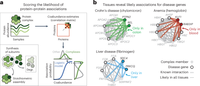
Association atlas reveals cell-type-specific associations

To explore cell-type-specific associations in our association atlas, we took the AP2 adaptor complex as a well-known example. The AP2 complex has neuron-specific functions in addition to functions that are general to all cells83. Indeed, the subunits of the AP2 complex were coabundant in all tissues (average association score between subunits = 0.80). We found 91 proteins that had association scores with all AP2 subunits in all tissues and were known to associate with AP2 (STRING score > 400). Among these, the 51 synaptic proteins (SynGO84) had higher association scores with the AP2 complex in the brain (average score = 0.54) compared to the other tissues (average score = 0.48 ± 0.00, P = 6.7 × 10−6, according to a one-sided Mann–Whitney U-test). Conversely, the nonsynaptic interactors had lower association scores with the AP2 complex in the brain (average score = 0.33) compared to the other tissues (average score = 0.43 ± 0.00, P = 1.1 × 10−21, according to a one-sided Mann–Whitney U-test) (Fig. 3a). We explored further examples by focusing on cell-type-specific associations in the context of disease. We found that proteins of hemoglobin are related to anemia and have likely associations with anemia proteins but only in the blood (Fig. 3b and Methods). Likewise, we found that subunits of chylomicron, which transports dairy lipids from the intestines, contain and have likely associations with proteins related to Crohn’s disease but only in the colon85,86. Lastly, we found that subunits of fibrinogen, synthesized in the liver, contain and have liver-only likely associations with proteins related to liver disease87,88. For the other tissues, we could find many examples of tissue-specific and cell-type-specific associations for protein complexes, cellular components and disorders such as diabetes and asthma (Supplementary Fig. 18). These examples demonstrate that our association atlas can be used to study tissue-specific functions of protein complexes and context-dependent associations for disease genes.

Fig. 3: Association scores define relationships between protein sets.

a, Association scores between AP2 subunits and known AP2 interactors (STRING scores > 400) that are synaptic proteins (NECAP1 and BIN1; SynGO) or not (DAB2 and NECAP2). Heat maps show association scores in the brain and averaged association scores for the other tissues. b, Associations of hemoglobin (GO:0005833) to anemia, chylomicron (GO:0042627) to Crohn’s disease and fibrinogen (GO:0005577) to liver disease. Proteins (nodes) are complex members (gray) and disease genes (black edge). Associations are likely in all tissues (thin gray lines) or likely in a single tissue and not likely in all others (thick colored lines). Thick gray lines are associations with prior evidence (STRING scores > 400). Disease genes defined through OTAR (Methods). c, Schematic of approach. Relationships are scored by aggregating the association scores between all pairs of proteins from disjoint sets. d, Relationship scores of cellular components (light gray; GO), GWAS traits (dark blue; OTAR L2G ≥ 0.5) and between traits and components (light blue). Each dot represents the relationship between two sets, indicating the average and CV of relationship scores relative to the tissue median. Green dots show relations of the ribosome and spliceosome (score > 1.75; green box); purple dots show relations of synaptic components (CV > 0.4; purple box). Comp., component. e, Dendrograms of the 15 most brain-specific GWAS traits (left) and the 15 GO cellular components having the most brain-specific relationship with OCD (L2G ≥ 0.5; right). Dendrograms were constructed with complete-linkage clustering using the Manhattan distance on the relationship scores between traits (left) or between cellular components (right). Heat maps show genes overlapping between cellular components and OCD (orange; Jaccard index) or the enrichment of nonoverlapping genes from cellular components with drug targets, genes associated with OCD in mice or genes less confidently linked to OCD through GWAS (purple–green; conditional log2 odds ratios of one-sided Fisher exact test; dots show BH-adjusted P values < 0.05; Methods). SV, synaptic vesicle; CCV, clathrin-coated vesicle; m., membrane; SC, Schaffer collateral; ASD, autism spectrum disorder.

Source data

Tissue-specific relations of traits and cellular components

We sought to generalize these examples of context-specific associations by systematically mapping the relationships amongst traits and multiprotein structures such as complexes or cellular components. As sets of proteins, we defined cellular components by Gene Ontology (GO) and defined human traits on the basis of the genome-wide association studies (GWAS) Open Targets (OTAR) locus-to-gene (L2G) score (≥0.5)89,90,91. We then scored the relationship between sets of proteins with the median association score of all possible protein pairs between the sets (Fig. 3c, schematic, omitting the intersection between gene sets). In total, we scored the relationships between traits (107,306 pairs), between traits and cellular components (240,967 pairs) and between components (134,002 pairs) across all tissues (Fig. 3d and Supplementary Tables 2–4). The relationship scores that were high in all tissues were primarily of core cellular components such as the ribosome and spliceosome (72% of relationships with relative average score > 1.75), while the relationship scores that varied most across tissues often involved tissue-specific structures such as synaptic components (61% of relationships with a coefficient of variation (CV) > 0.4). These observations suggest that the relationship scores recapitulate the relatedness of protein sets in a tissue-specific manner, particularly for the brain.

Relationship scores for prioritizing disease genes

Additionally, we unbiasedly scored the tissue specificity of each protein set as the median association score between all pairs of its proteins (Methods and Supplementary Tables 5 and 6). Using these scores, we then selected the 15 traits most specific to the brain, 13 of which were indeed related to the brain (Supplementary Table 7). Clustering these traits using the trait–trait relationship scores from the brain revealed a hierarchical organization of traits with co-occurring conditions such as anorexia nervosa, obsessive–compulsive disorder (OCD) and Tourette syndrome closely clustering together92,93 (Fig. 3e, left dendrogram). As an example, we further determined the 15 cellular components that had the strongest brain-specific relationships with OCD, all but one of which were related or specific to neurons (Fig. 3e, right dendrogram, and Methods). The majority of these cellular components had few genes in common with the genes confidently associated with OCD (Fig. 3e, orange heat map; Jaccard indices < 0.04). However, after removing the few genes confidently associated with OCD through GWAS, we found that almost all components were still enriched with or contained OCD-related genes (Fig. 3e, purple–green heat maps), that is, drug targets for OCD (odds ratio = 8.4 ± 1.8; ChEMBL clinical stage 2 or higher)