Datasets

To evaluate the effectiveness of our method, scRNA-seq datasets with multiple batches from different biological systems are collected and input into our model enrolled. Notably, these datasets encompass cell clusters with known differentiation directions, allowing us to validate the accuracy of our estimated velocity through visualization plots and metric values. The data statistics are shown in (Table 5) and are described as follows.

The dataset comprising neural-related cells from mouse spinal cord injury (SCI) tissue was derived from two sources: the GEO database and our own experimental data labeled as "xj". The GEO dataset, accessible under the accession number GSE162610, was generated using the 10X Genomics platform. On the other hand, the xj dataset was obtained through sequencing on the BD Rhapsody platform and will be made available in the near future. For the purpose of detecting latent differential relationships, only neural-related cells were selected from mouse spinal cord injury (SCI) tissue for analysis. The dataset named “SCI1” exclusively contains the GEO dataset, while the dataset named “SCI2” contains the GEO dataset and xj dataset.

The spinal cord dataset with multiple time-series batches is downloaded from GSE189070 and sequenced from the 10X genomics platform. The immune-related cells are selected to detect the latent differential relationship. The dataset is named as “SCI3” in the work.

The olfactory bulb dataset will be released in the near future and sequenced from the BD Rhapsody platform. The neural-related cells are selected to detect the latent differential relationship. The dataset is named “olfactory bulb” in the work.

The above datasets need to be processed upstream to get spliced/unspliced expression matrix from fastq files, where velocyto [3] is used after cellranger 6.1.2 for the 10X genomics platform or rhapsody 1.10 for the BD Rhapsody platform. The following datasets can be accessible as spliced/unspliced expression matrix format directly.

The “Dentate gyrus” dataset is one of the most classical datasets for RNA velocity tasks that can be directly downloaded from scVelo packages with scvelo.datasets.dentategyrus. The transition from OPC (oligodendrocyte progenitor cell) to OL (oligodendrocyte) is the known differentiation direction that is accurately estimated by our method.

The “Mef reprogramming” dataset is the result of one of the first methods for designing time-series RNA-seq experiments and preprocessed [13]. The time series batches of the dataset are 0, 2, 5, and 22 days after reprogramming. The known transition is from mouse embryonic fibroblasts (MEF) to neuronal cells that are expressed as “mef → day 2 intermediate → day 2 Ascl1-induced → day 5 intermediate → day 5 early induced neuronal cells → neuron.”

The mouse “Gastrulation” and “Gastrulation erythroid” datasets are both from the scVelo package with scvelo.datasets.gastrulation and scvelo.datasets.gastrulation_erythroid., where the batch interval is 0.25 day which is so small that the K-nearest neighbors for all total dataset is more suitable for better result (Table 5).

Table 5 Datasets overviewData preprocessing

The pre-processing module of all datasets analyzed in this paper does not fully follow the standard procedure of scanpy packages since it is necessary to preprocess both spliced and unspliced count matrices at the same time. The preprocessing part is divided into two major steps as a whole.

The first step is quality control and data transformation. Firstly, high-quality genes are retained that are expressed in at least 20 cells in both spliced and unspliced count matrix. Secondly, the matrix is normalized such that the sum of all gene expressions in each cell is the same value, which is the median of all cell expressions. Then, the first 2000 highly variable genes are extracted to accelerate subsequent analyses. Finally, log scaling is performed. The above operations can be implemented by calling scvelo.pp.filter_and_normalize in the scvelo package.

The second step is feature reduction and neighborhood construction. Firstly, principal component analysis (PCA) reduces the feature dimension to accelerate later preprocessing operations. Then, the Euclidean distance matrices are calculated for cells within the same batch or between batches at adjacent time points. The asymmetric distance matrices are transferred to symmetric probability matrices. Next, KNN constructions are used for cells within the same batch and MNN constructions based on optimal transfer are used for cells in adjacent time batches, respectively. Finally, the local graph structure constructed multiple times is concatenated together to become the global overall graph structure. The relevant formulas are shown below.

$$p_^} = \exp ( - (d(x_^} ,x_^} ) - \rho_^} )/\sigma_^} )$$

(1)

$$p_^} = (p_^} + p_^} ) - p_^} \cdot p_^}$$

(2)

The bidirectional transition probabilities \(p_^}\) between cells \(i\) and \(j\) can be calculated based on the unidirectional probabilities \(p_^}\) from cell \(i\) to cell \(j\) and \(p_^}\) from cell \(j\) to cell \(i\), following Eq. (3). However, due to the distinct meanings of the two types of edges, their calculation methods also differ. For intra-batch k-nearest neighbors (KNN) construction, the default sc.pp.neighbor function provided by scanpy can be utilized with the method described in (4), where \(\rho_^}\) and \(\sigma_^}\) are scaling parameters. For inter-batch mutual nearest neighbors (MNN) construction, the POT package can be used to pass the distance matrix (denoted as “distance”) between batches a and b, and ot.emd(Ia, Ib, distances) can be called to obtain the optimal transfer probabilities matrix. For this matrix, we retain the top K values that represent the highest mutual transition probabilities between each pair of cells.

Parameter inference of VeloVGI

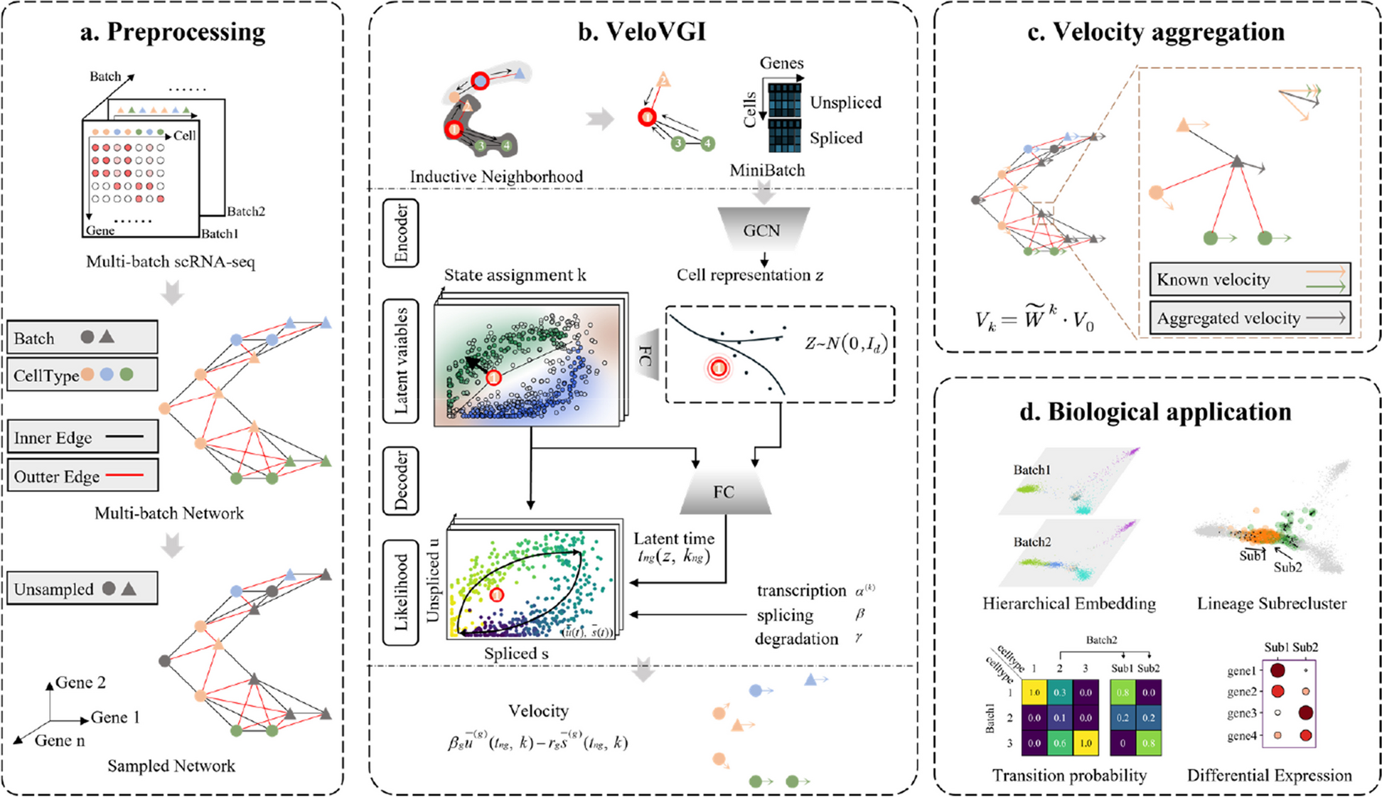
Several models based on the Variational Autoencoder (VAE) framework have been proposed for RNA velocity analysis in single-cell omics data. Notable examples include VeloVAE [10], Pyro-Velocity [11], LatentVelo [12] and VeloVI [24]. The VAE models have demonstrated its effectiveness in removing batch effects [22], making it a valuable tool for analyzing scRNA-seq data. In this study, the VeloVGI model, estimating RNA velocity parameters, is based on VeloVI due to its efficient implementation in scvi-tools [31], a Python library designed for probabilistic analysis of single-cell omics data which is easy to deploy and redevelop.

The specific estimation process of VeloVI is centered around VAE. The concatenated matrix \((U,S)\), formed by combining the spliced matrix \(S\) and the unspliced matrix \(U\), serves as the input for the model. The encoder fits the distribution of features and resamples to obtain the hidden layer representation of cells. The decoder first uses this embedding to fit the parameters of the transcription rate and the state of the cell and then uses the basic RNA velocity assumptions and the derived formulas for cell and gene specificity to fit the estimated \((\hat,\hat)\). Finally, the model is trained by minimizing MSE (mean square error) through gradient descent. The transcription \(\alpha\), splicing \(\beta\), and degradation \(\gamma\) parameters conform to the differential equations of a kinetic model. These parameters are estimated by fitting the decoder of a variational autoencoder (VAE) as an auxiliary task, and the velocity is computed using the estimated parameters by formula (6).

$$\begin \frac} = \alpha^ (t) - \beta u(t) \hfill \\ \frac} = \beta u(t) - \gamma s(t) \hfill \\ \end$$

(3)

$$v^ (t,k) = \frac^ (t,k)}} = \beta_ \overline^ (t,k) - \gamma_ \overline^ (t,k)$$

(4)

VeloVGI adds a graph representation learning strategy in the encoder section based on it, fully utilizing neighbor relationships to enhance the model's representation ability, as described in the next section.

Graph learning representationGCN

Graph convolution network (GCN) [32] is primarily designed to extract the latent representation of nodes by combining the original feature of nodes and neighbor relationships, which can be conducted in matrix form as

$$^=}^}\widetilde}^}^^ where ^=concat(U,S)$$

(5)

The formula consists of message generation and message aggregation. Message generation is expressed as \(^^\) where \(^\) and \(^\) correspond to feature and weight in \(l\)-th layer of model. Message aggregation is represented as \(}^}\widetilde}^}\) where \(\widetilde=W+_\epsilon ^\) based weighted adjacency matrix \(w\) additionally adds self-loops and \(\tilde\) is the degree matrix of \(\widetilde\). The formula as a whole implements the feature transformation \(^\) from layer \(l\) to layer \(l+1\) while \(^\) matrix is the concatenation of unspliced \(w\) (the fomulation variable w should be deleted, I can't do that) count matrix \(U\) and spliced count matrix S.

MiniBatch, GraphSAGE

Since scRNA-seq datasets from tissue samples are usually composed of multiple batches and the number of cells may be in the tens or even hundreds of thousands, using GPU for training becomes extremely resource-intensive if all cell features and neighbor relationship graphs are input into the model simultaneously. Therefore, a minibatch strategy for the graph is needed to split the whole graph into many subgraphs to train the model. A simple random sampled minibatch is not suitable for this task, which results in the loss of a large number of neighbor relationships while every minibatch should preserve sufficient neighbor relationships for model training. After trying many other strategies, an inductive representation learning and neighborhood sampling method called GraphSAGE [23] was found to be well-suited for this task. This strategy, after sampling randomly selected nodes, extends to their surrounding neighbors and generates a directed graph for subsequent message aggregation. The number of neighbors for each GCN layer and the GCN layer count can be adjusted as needed.

The implementation of this graph learning representation part is mainly based on PyTorch Geometric [33].

Sample and recovery strategySample

The presence of a large number of cells is a notable characteristic of multi-batch datasets. In addition to the previously mentioned minibatch strategy to reduce resource pressure in feature extraction, down-sampling during preprocessing can also effectively compress the dataset size and reduce resource consumption. Regarding the specific sampling method, we discovered that random sampling is straightforward and effective after experimenting with various methods, including node centrality sampling.

Recovery

For cells that have not been sampled, their velocity-related properties (including the velocity vectors in both high and low dimensions, the relevant parameters in the underlying assumptions, etc.) can be obtained by calculating the average of the corresponding properties of the sampled neighboring cells as

$$V_ = \tilde^ \cdot V_$$

(6)

This process is similar to the moment operation in the scVelo package preprocessing process.

Lineage subcluster

The typical subcluster based on gene expression values often involves subjective decisions when determining whether further sub-clustering is necessary. It requires choices of resolution and cluster number without clear reference. In this regard, lineage subcluster offers a solution to these challenges. When accurate velocity stream plots are available, some cellular clusters may clearly exhibit multiple distinct differentiation trends. For example, as seen in Fig. 2a, NSCs exhibit two distinct subgroups. This observation indicates the presence of various differentiation potentials within these clusters, a phenomenon we term lineage re-cluster. These lineage subclusters are defined based on the differentiation direction presented in the lineage or developmental trajectory.

The method for identifying lineage subgroups is straightforward. Firstly, it is necessary to determine which major clusters have the potential for lineage subgroups. This assessment can be made by observing the velocity stream to determine whether a particular cluster exhibits consistent and gradual changes in velocity vectors. In this context, “consistency” can be inferred by examining whether the in-cluster coherence (ICVCoh) metric of the major cluster is sufficiently large. The concept of “gradual changes” can be evaluated by measuring the similarity between the velocity vectors of all cells within the major cluster and the average velocity vector of the cluster.

Next, the specific segmentation of lineage subgroups needs to be established. In this context, we perform conduct clustering on concatenated features \(X_ = [V_ ,X_ ]\). The optimal number of clusters for lineage subgroups is determined by selecting the clustering solution with the highest silhouette coefficient. This process enhances the accuracy of identifying the structure of lineage subgroups.

Evaluation metric

The differentiation relationship in the biological background, which plays a significant role in RNA velocity result assessment, can evaluate the validity of RNA velocity methods on a reduced dimensional visualization graph such as UMAP or tSNE. Furthermore, cross-boundary direction correctness (CBDir) and in-cluster coherence (ICVCoh) are currently recognized as relatively reliable evaluation metrics that transform fuzzy visualizations into precise values [7, 8]. To elaborate, CBDir measures cosine similarity of velocity and expression difference among neighbor cells on the ideal cluster differentiation boundary and specific direction within the heterogeneous cluster to evaluate how likely a cell can develop towards other neighbor target cells. ICVCoh, on the other hand, assesses velocity consistency among neighbor cells within the homogeneous cluster, representing the smoothness of cell velocity.

Boundary cells should be defined before computing CBDir, which requires pairs of cell clusters as input of ground truth development directions. Boundary cells from A to B represent the set \(}_\) as

$$}_ = \left\ |\exists c^ \in C_ \cap (c)} \right\}$$

(7)

The formula for computing the CBDir score is

$$}BDir(c) = \frac \in C_ \cap (c)} \right\}} \right|}}\sum\limits_ \in C_ \cap (c)}} - x_c} \right)}} \right| \cdot \left| - x_c} \right|}}}$$

(8)

The formula for computing the ICVCoh score is

$$ICVCoh(c) = \frac \in C_ \cap (c)} \right\}} \right|}}\sum\limits_ \in C_ \cap (c)}} }} \right| \cdot \left| } \right|}}}$$

(9)

In the above formula, \((c)\) is a set of neighbors of the cell \(c\) and \(x_\) represent the expression of the source cell \(c\) and target cell \(c^\) in low-dimensional space in UMAP, tSNE, or other embedding space.

However, in the real batch datasets, since the inter-batch neighbor relationships are much fewer than the intra-batch neighbor relationships, the two existing metrics may focus too much on intra-batch cell velocity performance and ignore the velocity results of batch effect integration. To address this issue, we improved on the two previous metrics by constructing BCBDir and BICVCoh to care only about inter-batch neighbor relationships and provide a more effective assessment of the performance of RNA velocity on datasets with batch effects. The slight modification is that the target cell \(c^\) should not belong to the same batch with source cell \(c\) represented as \(\tilde(c)\). The new boundary cell set \(}_^}}\), BCBDir, BICVCoh are as follows:

$$}_^}} = \left\ |\exists c^ \in C_ \cap (c) \cap \tilde(c)} \right\}$$

(10)

$$}BDir(c) = \frac \in C_ \cap (c) \cap \tilde(c)} \right\}} \right|}}\sum\limits_ |\exists c^ \in C_ \cap (c) \cap \tilde(c)}} - x_c} \right)}} \right| \cdot \left| - x_c} \right|}}}$$

(11)

$$BICVCoh(c) = \frac \in C_ \cap (c) \cap \tilde(c)} \right\}} \right|}}\sum\limits_ \in C_ \cap (c) \cap \tilde(c)}} }} \right| \cdot \left| } \right|}}}$$

(12)

Hardware configuration

This work’s hardware configuration is supported by a high-performance computing platform of Xidian University with GPU of A100 and V100s.