In this section, we provide a computation of a Brain Space obtained from a set of patients. In particular, to highlight differences between brain functional alterations due to different diseases, we choose patients from different healthcare datasets relating to different neurological disorders as listed in Table 2. We chose states of patients with healthy brains or with diseased brain, with features representative of the respective disorders. In particular, we focus on patients individually investigated for preliminary applications of the K-operator for specific disorders. Moreover, we chose the Anatomic Automatic Labeling 3 (AAL3) atlas (Rolls et al., 2020) and selected the 160 ROIs within all the fMRIs of the considered patients.

In Fig. 4, we can see the Brain Space generated for the patients in Table 2.

Fig. 4

A quantitative example of brain space for a selection of patients. For the explanation of the points’ labels, see Table 2 (right). The labels contain a weighted sum of the regions of interest, automatically computed (Table 3). The states belonging to the same patients are identified with the same symbol. The arrows, indicating time evolution, are added as post-processing

On the other hand, Fig. 5 shows the simplex (violet) of Alzheimer-Perusini’s patients and the simplex (blue) of Parkinson’s patients. As we can see, there is a clear separation between these disease subspaces.

Fig. 5

A quantitative example of brain space for the selected patients, where we also use the same symbol for the same patient, with the exception of the two normal ones, with the same symbol, an \(\times \) (limitation of the available marker shapes in 3D in Python). Here: Euclidean dissimilarity

As concerns the schizophrenic patient, he is distant from the PD patients and even more distant from the follow-up of one of the PD patients. This makes sense since the evolution of PD involves a defect of dopamine neurotransmitters due to damage in the substantia nigra, and a consequent deficit in dopamine is “opposed” to the excess of dopamine occurring in the same region for schizophrenic patients (van Hooijdonk et al., 2023).Footnote 2

The axes of Figs. 4 and 5 contain the synthetic description of MDS dimensions 1, 2, and 3. The MDS algorithm automatically computes a weighted sum of the contribution of each region of interest for each axis in terms of correlation values. The higher the ROI absolute value, the higher the impact of the ROI in the space separation between points.

It is worth noting that MDS is a dimension-reduction technique designed to project high-dimensional data down to lower dimensions while preserving relative distances between observations. Since in our example we reduce 160 ROIs to obtain a 3D representation of the Brain Space, the more points we add to the Brain Space, the more the axes values are refined.

Table 3 The first five ROIs more heavily affecting (in absolute value) the axis content of the brain space, before (left) and after (right) the inclusion of the last patient in Table 2

Table 3 shows the first five more impacting ROIs on each axis, before (left) and after (right) the addition of the last patient of Table 2. With a larger population, the classification could become more precise. Nevertheless, with this simple example, we also draw information on the feasibility of our brain state definition from a purely theoretical approach to a computational one.

The MDS are computed after the pairs of ROIs, the most influential to distinguish between brain states according to the \(\mathcal \) matrices. They can also be related to the single ROIs most influential in those pair variations. Our reported ROI correlations are still exploratory, but the analysis can be enriched with the features directly derived from the connectivity matrices. In fact, the individual impact of ROIs on an MDS axis is obtained via the sum of the contributions of all connections involving that ROI. And it includes a 1/2 factor, to avoid counting a pair of ROIs twice. By considering the impact of the “original” pairs of ROIs, we can listen the first of them according to their impact, as shown in Table 4, directly for the case study with all patients.

Table 4 The most influential pairs of ROIs

The MDS distribution is sensitive to the characteristics of inputted brain states. In fact, a progressive refinement can be achieved with the addition of more patients.

To complete the discussion of the brain space, we also give a quantitative representation of a path. Within the brain space, the progression of the disease is an arrow, labelled as the K-operator, transforming, for instance, the brain state of a Parkinsonian patient at the baseline (for example, PD_patB) to the state at the first follow-up (for example PD_patB_FU). If we consider a space of a number of dimensions equal to the number of ROIs, thus 160 in the present case, then the brain-state path from baseline to follow-up is perfectly described by the K-operator computed between the two states and for that choice of atlas. However, in these compressed dimensions via a multi-dimensional scaling, some ROIs will contribute more than others, depending on the other states in space, see Table 2. Then, the path under consideration will be described by a compressed version of the K-operator. By extracting the coordinates of the points PD_patB and PD_patB_FU, we can write:

$$\begin K|_\text :\,& PD\_patB \rightarrow PD\_patB\_FU \\ & \Rightarrow [-34.25, -15.81, -3.611]\rightarrow [-13.48,-47.21,-69.99]. \end}\end$$

(2)

Hence the path from PD_patB to PD_patB_FU can be computed as the percentage of variation of each of these ROIs. For the MDS Dimension 1 we have 60.64%, for Dimension 2 we have 198.61%, and finally for Dimension 3 we get 1838.24%. These percentage variations have to be reported on the five most influential ROIs and their correlation with the axes from Table 3. Limiting ourselves to the first ROIs for each axis, we can assess that the strongest alteration occurs for the third MDS dimension, and thus mostly impacting the first ROI of the list, cerebellum 7b right or the thalamus geniculate (considering the left or right side of Table 3), followed at large by the second MDS dimension with cerebellum 4R or frontal superior medial R, and the first MDS dimension, whose greater weight is constituted by precuneus left or fusiform right. However, due to the two orders of magnitude of the change in the third MDS dimension, also the other four ROIs that are impacting that axis are worthy of notice (temporal mid-left, temporal pole mid-left, cerebellum 7 right, and occipital mid-L).

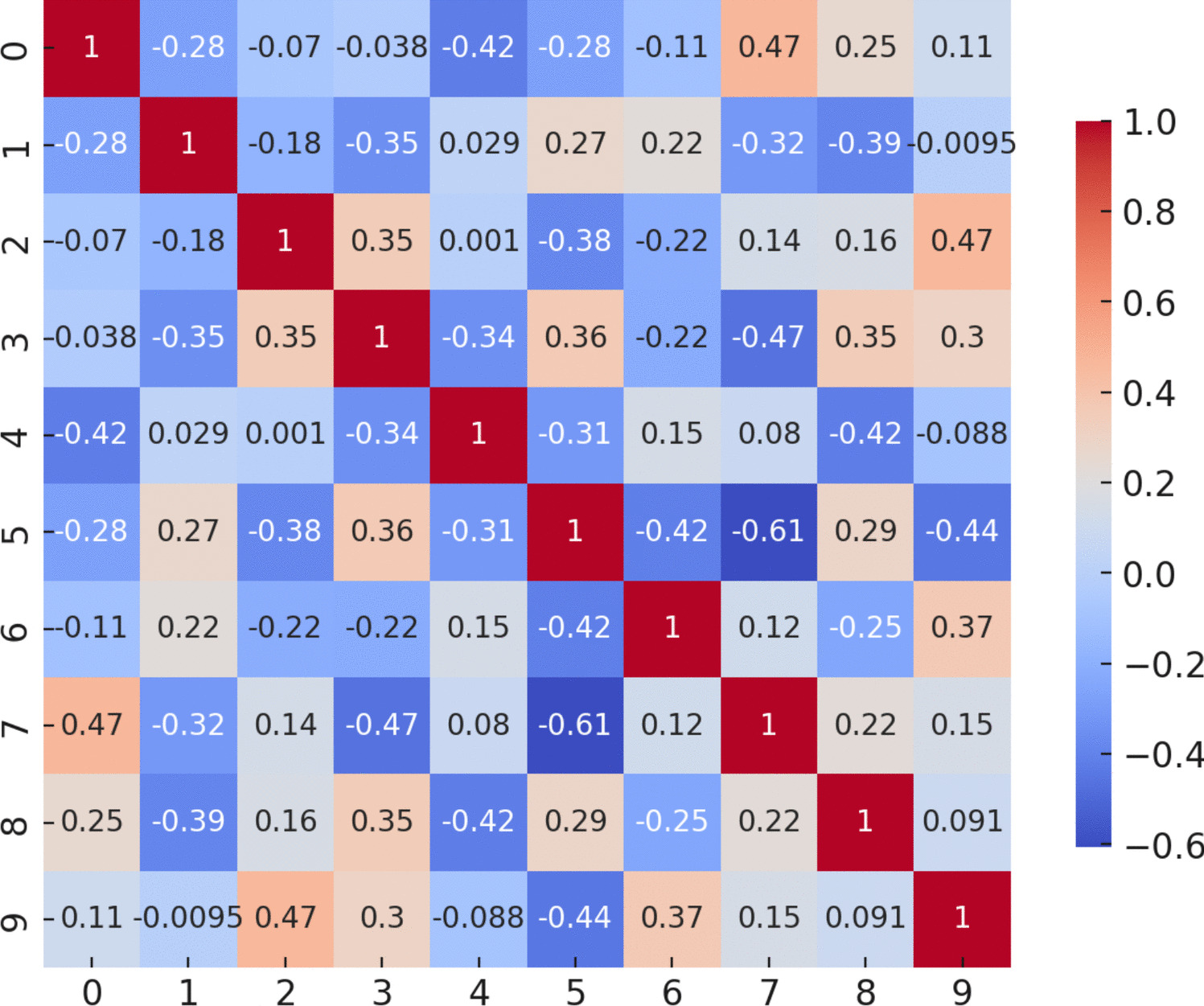
By looking at Fig. 6 taken from (Mannone et al., 2024c) representing the K-operator for the disease progression of patient B and highlighting the mentioned regions (with thicker lines for the first ROIs of the third dimension), we check that they correspond to specific clusters of (mostly blue, i.e., negative) points in the K-operator for the 160 ROIs.

Fig. 6

K-operator for the disease progression of patient B (Table 2), from the baseline to the first follow-up. The thicker lines indicate the first ROIs more correlated with the third MDS dimension, where the change from baseline to follow-up is higher. (Original figure taken from (Mannone et al., 2024c))

We can relate the coordinates of the two brain states connected by the considered K-operator to the most influential pairs of ROIs. In particular, we can focus on the third axis, the one where the higher change is found. We thus obtain the list of Table 5. In particular, we notice the pairs:

15-87 supplementary motor area, and temporal pole: superior temporal gyrus;

5-6, both middle frontal gyrus;

27-87 anterior orbital gyrus, and temporal pole: superior medial frontal gyrus,

and in particular the ROIs:

3: superior frontal gyrus,

35: anterior cingulate,

1: precentral gyrus,

37: middle cingulate gyrus,

84: Heschl’s gyrus,

70: angular.

From the evaluation of the complete K-operator (Figure 6), we can notice the impact of the nearby pairs of ROIs 89-21, 90-21, near to 15-87 and 27-87, and we can also notice, from visual inspection, the importance of the agglomerates around 5-6, and the small agglomerates in correspondence of 71-35. The highlighted areas, near to the regions of Table 5, are the following:

89: middle temporal gyrus,

21: superior frontal gyrus,

27: anterior orbital gyrus,

71: precuneus, and

35: anterior cingulate.

Summarising, the “classic” strategy for the computation of the K-operator is: ROIs\(\rightarrow \mathcal \)-matrices\(\rightarrow \) \(K\)-operator (without dimensional loss), while the strategy proposed in this article, to provide a computational example of construction of brain spaces, is: ROIs\(\rightarrow \) MDS \(\rightarrow \)positioning of \(\mathcal \)s as points in the brain space, and subsequently the computation of the K-operator within the reduced space.

Table 5 The most influential pairs of ROIs concerning the third axis, MDS dimension 3, where the higher change is highlighted for the considered example (patB, from baseline to the first follow-up)