The Young Finns Study (YFS) is an ongoing prospective follow-up study that has begun in 1980 (baseline assessment), and follow-ups have been conducted in 1983, 1986, 1989, 1992, 1997, 2001, 2007, 2011/2012, and 2018–2020. Altogether 4320 subjects were invited (born in 1962, 1965, 1968, 1971, 1974, or 1977), and 3596 of them participated in the baseline study. The sampling was designed to include a population-based sample of non-institutionalized Finnish children, representative with regard to most crucial sociodemographic factors. In practice, the sampling was conducted in collaboration of five Finnish universities with medical schools (i.e. Universities of Helsinki, Turku, Tampere, Oulu, and Kuopio). A more detailed description of the YFS can be found elsewhere [36].

Of the 3596 participants, we first excluded 1885 participants who had no data on epigenetic clocks. Later, participants were excluded if they had no data available on the sleep measure of interest or any of the covariates in a particular model. Out of participants who had data available on epigenetic clocks, 93 did not have data on minimal covariates, 250 had no data on all health covariates and 270 had no data on all socioeconomic covariates. The sample size varied between 1439 and 1618 in analyses regarding sleep measures, and between and 581 and 716 in analyses regarding shift work.

Epigenetic ages were calculated for blood samples from 2011. Genome-wide DNA methylation levels from whole blood were obtained with Illumina Infinium HumanMethylation450 BeadChip (n = 182) or Illumina Infinium MethylationEPIC BeadChip (n = 1529) following standard protocol by Illumina. Preprocessing and normalization of the methylation data have been described in detail elsewhere [37].

Indicators of epigenetic age included in the study were the Horvath clock [2], Hannum clock [1], PhenoAge [3] and GrimAge [4]. For all these clocks, we utilized the measure of epigenetic age deviation, which is defined as the residual that results from regressing epigenetic age on chronological age [38]. These are denoted as AgeDevHorvath, AgeDevHannum, AgeDevPheno, and AgeDevGrim. We also included a measure for pace of ageing, DunedinPACE [5]. In sensitivity analyses, we used the derivatives of the Horvath and Hannum clocks, IEAAHorvath, IEAAHannum, and EEAAHannum [38] as well as principal component (PC)-based epigenetic clocks including AgeDevPCPheno, AgeDevPCGrim, AgeDevPCHannum, and AgeDevPCHorvath [39]. All measures of epigenetic age deviation or pace of epigenetic ageing were calculated according to published methods described above. Pearson correlations between different measures of epigenetic ageing can be found in Supplementary Fig. 1.

Participant responses for all sleep measures (except for circadian rhythm lateness) were gathered in both 2007 and 2011. In the final analyses, we used the average scores between the measurement years because, first, also previous studies on sleep and epigenetic ageing have averaged sleep scores if data was available on multiple measurement years [22]. Second, evidence from intervention studies suggests that lifestyle factors need to be examined over periods of years to observe changes in epigenetic clocks [40]. Third, because there were some missing values in 2007 and 2011, using the average scores allowed us to increase the sample size and thereby the statistical power of our analyses.

Insomnia symptoms were measured using Jenkins Sleep Scale (JSS) [41] in 2007 and 2011, capturing the frequency and severity of symptoms. JSS includes four items (e.g. “During the past month, how often have you experienced trouble falling asleep?”) with a 6-point Likert scale (1 = “not at all”, 6 = “every night”). JSS has demonstrated high internal consistency and its reliability and construct validity appear to be good [42]. Additionally, the JSS has shown good predictive validity in various health outcomes, including weight gain [43] and type II diabetes [15]. The Finnish translation of the JSS is also found to have adequate internal consistency and construct validity in a previous cohort study [44]. In this study, an averaged score of the JSS items was calculated for 2007 and 2011 separately (if the participant had responded to at least 50% of the items), with higher scores indicating more severe insomnia symptoms. Then, the scores for both years were averaged. If the score for only one year was available, it was used instead. The value of Cronbach’s alpha was α = 0.77 in the 2007 survey and α = 0.76 in the 2011 survey, indicating high consistency between items in both surveys and thus sufficient reliability. Participants’ scores in 2007 and 2011 showed moderate correlation (Pearson’s r = 0.54, p < 0.001), indicating moderate stability.

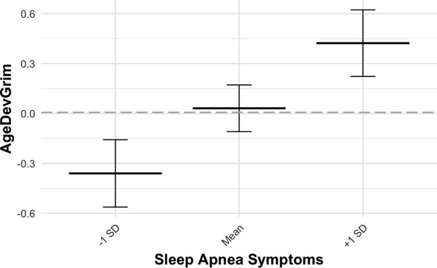
Symptoms of obstructive sleep apnoea were measured using Epworth Sleepiness Scale (ESS) [45] and three additional items more specific to obstructive sleep apnoea. ESS measures excessive daytime sleepiness, which can be related to disorders such as obstructive sleep apnoea and narcolepsy. ESS was used in follow-ups of 2007 and 2011, and it includes eight items measuring the tendency to fall asleep in various everyday situations (e.g. “How likely will you fall asleep when you are watching TV?”), and answers are given with a 4-point Likert scale (0 = “I would never doze”, 4 = “a high chance of dozing”). The internal consistency of the ESS has been found to be good [46]. In our sample, the Cronbach’s alpha for ESS was α = 0.72 in both 2007 and 2011, indicating high consistency between items. ESS has previously correlated with other measures of sleep apnoea and the measure seems to have good test–retest reliability in non-clinical samples [47]. In addition to the items of the ESS, three other items from 2007 and 2011 were included in the sleep apnoea symptom measure of this study. They were related to frequency of snoring (1 = “once a month or less”, 5 = “every night or nearly every night”), quality of snoring (1 = “I do not snore”, 5 = “loud and uneven snoring”) and frequency of episodes of stopped breathing during sleep (1 = “once a month or less”, 5 = “every night or nearly every night”). Average scores of the eight ESS items were calculated for 2007 and 2011, with higher scores indicating more severe symptoms. The scores of 2007 and 2011 were then averaged. The same process was then repeated for the three additional items. Then, the ESS average and the average score of the three other items were standardized. Finally, the two standardized scores were averaged. Participants were excluded from analyses if responses were unavailable for more than 50% of items in both years. Participants’ sleep apnoea symptoms scores in 2007 and 2011 showed high correlation (Pearson’s r = 0.73, p < 0.001), indicating high stability.

A sleep deprivation score was computed for both 2007 and 2011 as the difference between self-reported optimal amount of sleep and actual amount of sleep. For the latter, participants were instructed to report their usual amount of sleep (reported as 5 h or less, 6 h, 6.5 h… 10 h or more). Scores for both years were then averaged. Existing evidence suggests that both sleep deprivation and excessive sleeping may be associated with poor health outcomes, including diabetes [48], indicating curvilinear associations between sleep deprivation and health outcomes. A curvilinear association has been reported when examining sleep deprivation and phenotypic age [49]. Therefore, the sleep deprivation score was also squared (with high values indicating both sleep deprivation and hypersomnia) and used as a quadratic term in additional models. In addition, we utilized a measure of sleep duration, calculated as the average of actual amount of sleep in 2007 and 2011. The responses between the measurement years showed moderate stability (Pearson’s r = 0.43, p < 0.001, and Pearson’s r = 0.56, p < 0.001, for sleep deprivation and sleep duration, respectively).

Circadian rhythm lateness was measured with a shortened version of the Morningness-Eveningness Questionnaire (MEQ) [50]. The predictive validity of MEQ is good since it has been found to be associated with various metabolic biomarkers among those with type II diabetes [51] as well as health behaviours and cardiovascular health among women [52]. The measure used in this study includes six selected items from the MEQ (items 4, 5, 9, 15, 17, and 19; e.g. “How easy do you find it to wake up in the morning (when you are not woken up unexpectedly)?”) and responses were given using a 4- or 5-point Likert scale (five items and one item, respectively). Responses were available from 2011, and the value for Cronbach’s alpha was α = 0.81, indicating high consistency between items. Each item was first standardized. Then, an average score was calculated for all available items so that higher scores indicate a later circadian rhythm. Participants were excluded from analyses if they had no available data for 50% or more of items. Pearson correlations between different sleep measures can be found in Supplementary Fig. 1.

The data on all covariates were gathered in 2011. All our models were adjusted for sex, self-reported smoking status (daily smoking vs. not) and DNA array type as these have been found to be associated with differences in DNA methylation and the pace of epigenetic age acceleration [6]. In addition, we utilized a set of health-related and socioeconomic covariates as described below.

A Physical activity index was based on a questionnaire including questions on the frequency and intensity of physical activity, frequency of vigorous physical activity, time spent on vigorous exercise (in hours), participation in organized physical activity, and average duration of a physical activity session. A more detailed description of the index and its creation can be found elsewhere [53].

To construct an alcohol consumption index, participants were asked to report their consumption of different alcohol beverages during the past week. The volumes were then summed to determine consumption measured in alcohol units (1 unit = 14 g of alcohol). The final categorization was done based on daily alcohol consumption (average of the week) as follows: 1: no alcohol consumption during the past week, 2: > 0 to < 2 units per day, 3: 2 to < 4 units per day, and 4: ≥ 4 units per day. The creation of this alcohol consumption index has been described in more detail elsewhere [54].

Other health covariates included diagnosed hypertension, systolic blood pressure, diastolic blood pressure, cardiovascular disease status, diabetes, and BMI. Diagnosed hypertension was self-reported by participants (0 = no, 1 = yes). Diastolic and systolic blood pressure were also included as covariates in order to better account for possible undiagnosed cases of hypertension. Blood pressure was measured in sitting position after 5-min rest. A mercury sphygmomanometer at phases 1 and 2 and with a random zero sphygmomanometer (Hawksley & Sons Ltd) at phase 3 was used. Cuff size for the measurement covered two-thirds of the participant’s arm length. Korotkoff’s first phase was determined as the indicator of systolic blood pressure. Readings to the nearest even number of millimetres of mercury were conducted 3 times for each participant. In the analyses, the average values of diastolic and systolic blood pressure were used between the three measurements. Cardiovascular disease status was considered positive (= 1) if the participant self-reported a history of stroke, chest pain related to coronary heart disease, congestive heart failure, coronary artery bypass surgery, or coronary angioplasty (all reported as 0 = no, 1 = yes). Otherwise, cardiovascular disease status was coded as 0. Diabetes was also self-reported and included in models separately (0 = no, 1 = yes). Separate items for type I and type II diabetes were combined: if either of these was reported as 1, the diabetes variable was coded as positive.

Socioeconomic covariates included gross yearly income, years of education and working hours (regular daytime job vs. not), all of which were self-reported. Gross yearly income was reported with a 13-point Likert scale (1 =  < 5 000 €, 13 =  > 60 000€). The education variable indicates years of education, including years of vocational training. Working hours during the past 12 months were reported with six categories (regular daytime job, shift work with two rotating shifts, shift work with three rotating shifts, fixed evening or nighttime working hours, irregular working hours, and not working outside home). The variable of working hours was dichotomized: regular daytime job (= 0) or shift work (= 1), which included all other categories except those not working outside home (coded as missing). Thus, those not working outside home were excluded from models where working hours were included as a covariate. In analyses regarding shift work, a measure of years in shift work was used. Participants freely self-reported the total amount of years they have spent in shift work. This resulted in a range of 0–30 years.

All analyses were conducted using R (versions 4.3.1 and 4.4.0). Stata MP 18.0 was used for plotting.

The associations between the sleep measures and epigenetic ageing measures were examined with linear regression models. Separate models were estimated for each epigenetic ageing measure (AgeDevHannum, AgeDevHorvath, AgeDevPheno, AgeDevGrim, and DunedinPACE). Each sleep measure was added as predictor separately (insomnia symptoms, sleep apnoea symptoms, sleep deprivation, and circadian rhythm lateness). There is evidence that health-related and socioeconomic factors seem to mediate the association between sleep and health [55]. Accordingly, to gain insight into possible mediating mechanisms between sleep disturbances and epigenetic ageing, we ran the regression analyses using three models with partially different sets of covariates (Models 1, 2, and 3). Model 1 only included minimal covariates (sex, daily smoking status, and DNA array type). Model 2 was additionally adjusted for health variables (BMI, cardiovascular disease status, diabetes, hypertension, systolic and diastolic blood pressure, alcohol use, and physical activity). Model 3 was adjusted for minimal covariates and socioeconomic covariates (gross yearly income, years of education, and regular daytime job vs. shift work).

To account for multiple testing, we used the false discovery rate (FDR) correction with the Benjamini–Hochberg method to adjust p-values [56]. The analyses were conducted for the whole sample, as no statistically significant sex interactions were observed while examining the associations between sleep measures and epigenetic ageing (p > 0.05).

Next, we examined whether years in shift work modify the associations between sleep measures and epigenetic ageing. Separate models were again estimated for each sleep measure. An interaction term between each sleep measure and years in shift work was added to the models, utilizing the same sets of covariates (Models 1, 2 and 3).

In order to assess the robustness of the results, the analyses were repeated using only cases where Illumina Infinium MethylationEPIC BeadChip was used for DNA methylation profiling. Additionally, the main analyses were repeated with IEAAHannum, IEAAHorvath, and EEAAHannum and four principal component (PC)-based clocks designed for reduction in technical noise and increased reliability [39]. These are denoted as AgeDevPCPheno, AgeDevPCGrim, AgeDevPCHannum, and AgeDevPCHorvath.

Attrition over the follow-up period was examined in order to evaluate possible differences between included and dropped-out participants. This was done using independent samples t-tests (for continuous variables) and chi-square tests (for categorical variables).