Source population

We used data from the Sustainable UNiversity Life (SUN) cohort study, described in detail in the study protocol [26]. Eligible participants were undergraduate or graduate (including up to masters’ level) full-time students at eight universities in and around Stockholm and Örebro with at least one academic year left until graduation. The targeted universities constitute a convenience sample, aiming to represent a variety of different university programmes.

Study sample, recruitment, and data collection

Eligible students were informed about the study during in-class presentations by study staff and/or by an email with a link to the first web-survey. Students who agreed to participate were followed every three months for one year with web-surveys, giving a total of five time-points of data collection. Data collection was ongoing between August 19, 2019, and December 15, 2021. For each survey that the participants filled out, they received a one-month free pass at a health club.

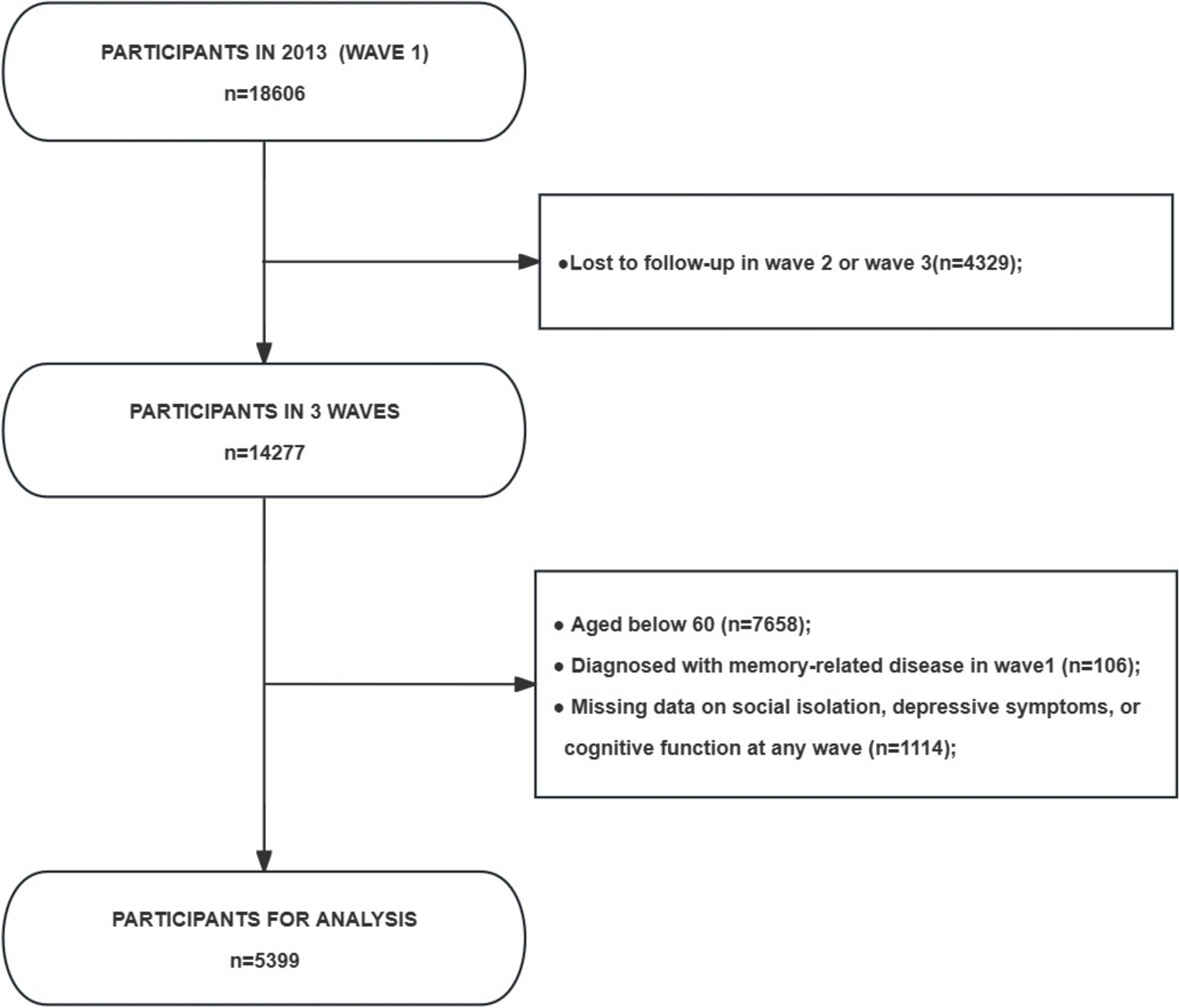
In the current analysis, we refer to the first time-point of data collection as pre-baseline, which was used for the measurements of potential confounders. The second time-point is referred to as baseline and used for exposure measurements. The third, fourth and fifth time-point, referred to as the 3-month, 6-month, and 9-month follow-up (FU3, FU6, FU9) with the figures representing months since baseline, were used for outcome measurements (Fig. 1). The study includes all women and men participating in the SUN cohort study and responding at baseline (n = 3503). Of those, 85% (n = 2982) responded at FU3, 78% (n = 2729) at FU6 and 73% (n = 2572) at FU9. Participants stating a gender identity other than woman or men were excluded from the study (n = 22) (Fig. 1).

Fig. 1

Flowchart of the inclusion of participants. Response rates are presented in relation to the baseline time-point. Participants were allowed to respond to later surveys even if they had missed earlier surveys and non-responders at each follow-ups are presented as number of persons not responding in relation to the baseline time-point. M = Men, W = Women

MeasuresExposures

SHV was measured at both pre-baseline (SHV0 in Fig. 2) and baseline. (SHV1 in Fig. 2). The recall period was one year at pre-baseline and three months at baseline (indicating if they had experienced sexual harassment since pre-baseline). Baseline measures were used as the exposures and pre-baseline measures as covariates.

Sexual harassment (wide subjective definition)

was measured by letting participants read the statement “According to the Discrimination Act, sexual harassment is an act that violates someone’s dignity and is of a sexual nature. Some examples of sexual harassment: groping or other unwelcome sexual touches, unwelcome sexual allusions, comments or suggestions, sexualized jokes and the spread of pornographic images or texts.” Participants answered by responding “Yes” or “No” to the following question: “Have you during the last year/previous three months experienced that you have been sexually harassed according to the definition above?”. Consequently, this item corresponds to the respondents subjective interpretation of what kinds of acts should be considered sexual harassment [3].

Specific forms of sexual harassment and violence

were measured using six items from the Sexual Experiences Questionnaire (SEQ) [2] that were modified for the Swedish context (Table 1). All items were answered on a five-point Likert scale from “Never” to “Very often”. The items covered: (1) offensive sexual remarks, (2) unwanted sexual attention, (3) presentation or distribution of sexist material, (4) uncomfortable touching, (5) beeing offered benefits for sex and (6) sex against ones will. The SEQ has shown adequate criterion validity and internal consistency (Cronbach’s α = 0.92) in student samples when used as a full scale [27]. In the current analyses each item was instead treated as a separate exposure, with exposure defined as responding “Once”, “Sometimes”, “Often”, or “Very often”, and non-exposure as responding “Never”, for each item respectively (Table 1). By using single items rather than scale scores, we can estimate the specific associations between exposure to different forms of SHV and symptoms of depression and anxiety, which would not be possible when using composite score [28, 29]. However, the downside of this approach is that the psychometric properties of individuals item of the SEQ are not known.

Table 1 Items used to assess exposure to sexual harassment and violenceOutcomes

Depression and anxiety symptoms were measured using the short-form Depression, Anxiety and Stress Scale (DASS-21) [30]. The scale consists of 21 items covering the three subscales Depression, Anxiety and Stress, with seven items each. The items are rated on a four-point scale from 0 (“Did not apply to me at all”) to 3 (“Applied to me very much, or most of the time”). The items of each subscale are summed to give subscale scores ranging 0–21. We used only the Depression and Anxiety subscales. DASS-21 has shown good psychometric properties among Swedish university students [31]. In the current sample, Cronbach’s alpha at pre-baseline was 0.91 for the Depression subscale and 0.79 for the Anxiety subscale.

Potential confounders

Covariates were selected based on previous literature [4, 7, 12, 13]. We used covariates measured at pre-baseline to ensure that none were on the causal pathway between the SHV exposures and the outcomes. We adjusted for the same covariates in all analyses; pre-baseline levels of all SHV exposures (dichotomous) and depression and anxiety symptoms (continuous), age (continuous), alcohol risk use (low, moderate or high risk alcohol use as defined by the Alcohol, Smoking and Substance Involvement Screening Test [32]), highest level of parental education (university level or below university level), place of birth (Sweden, Nordic countries, Europe, Outside Europe), study year (1st, 2nd, 3rd, > 3rd), education type (technical, medical/health, social science/humanities, economic, other) and civil status (single or partner). By adjusting for prior exposure and outcome levels, we aimed to separate the effect of recent exposure from that of prior exposure and prior outcome levels (Fig. 2). This approach may also reduce potential confounding from prior SHV, and depression and anxiety symptoms present before enrolment in the study (Fig. 2). With adjustment for prior exposure, estimates represents how changes in the exposure are associated with changes in the outcome [19, 33], such that it can be interpreted as the effect of incident rather than prevalent exposure [19]. It should be noted that the estimates aim at the effect of recent exposure, not to the accumulated effect of repeated exposure to SHV.

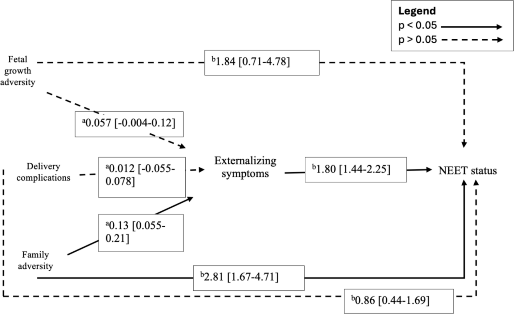
Fig. 2

Directed acyclic graph showing the assumed causal structure between sexual harassment and violence (SHV) and the outcomes (depression and anxiety symptoms) at different timepoints before and during the follow-up period. Yk denotes the outcome at follow-up k (FU3, FU6, FU9). SHVt denotes value of the exposure to SHV at time t (before enrolment, pre-baseline, baseline). C is a set of pre-baseline covariates including age, place of birth, parental education, type of education, study year, education type and civil status. The dashed arrows represent potentially biasing paths of direct long-term effects (not mediated through intermediate variables) that were not adjusted for in current analysis but assumed to be of little or no influence

Statistical analyses

Pre-baseline characteristics of the sample for women and men are presented in Table 2, as number and percentages or means and standard deviations (SD). Numbers of exposed to different forms of SHV at baseline is presented in Table 3 for women and men respectively.

The association between the SHV exposures and levels of depression and anxiety symptoms were estimated using Generalized Estimating Equations (GEE). We built separate models for each exposure-outcome combination, for women and men, respectively. All models were specified with independent working correlation structures, identity link functions and robust sandwich standard error estimators. Follow-up time was included in the models as a categoric variable with three levels (FU3, FU6 and FU9), and we included an interaction term between the exposure and follow-up time to let the association between exposure and outcome vary by the length of follow-up. This modelling approach is analogous to performing separate linear regression models for the outcomes at each follow-up time but has the advantage of providing a statistical test of whether the associations between exposure and the outcomes differs depending on the length of the follow-up.

All models were adjusted for pre-baseline covariates. For covariates assumed to have time-varying associations with the outcomes (i.e. pre-baseline SHV and depression and anxiety symptoms), we also included interaction terms with follow-up time.

Results are presented as the adjusted estimated mean differences (MD’s) of depression and anxiety symptoms between exposed and unexposed at each follow-up time, along with 95% confidence intervals (CI’s) (Table 3). For FU6 and FU9, where the estimated mean difference was the sum of the estimate for the exposure coefficient and the coefficient for its interaction with follow-up time, CI’s were calculated according to the formula provided by Figueiras, Domenech-Massons and Cadarso [34].

Sensitivity analysis

We had complete data on covariates and exposures for all 3503 participants, but data for the outcomes were missing for participants that were lost to follow-up (Fig. 1). GEEs with missing data are unbiased only if data is missing completely at random (MCAR). To assess the sensitivity of our estimates to the MCAR assumption, we imputed data for missing outcomes using multiple imputation (MI) by chained equations, creating 5 imputed datasets. Imputed values were predicted by all covariates and outcomes with a point-biserial correlation to missingness of at least 0.1, using predictive mean matching. All analyses were performed as described above in all imputed datasets, and estimates were pooled using Rubin’s rules (Online resource eTables 3 and 4). MI allows for the less restrictive missing at random assumption (i.e., that outcome data is missing at random conditional on the variables used to predict imputed values) and provides a sensitivity analysis for potential selection bias due to violations of the MCAR assumption.